21 Theory of ANOVA

ANOVA is called ANOVA because it analyses/breaks down/partitions the variance in our experiment. In essence, ANOVA takes the overall variability in scores in our experiment and breaks it down into a part that can be explained by the experimental manipulation (systematic variation), or what we’ll call “the model,” and the part that cannot be explained, that is due to extraneous variables (unsystematic variation).

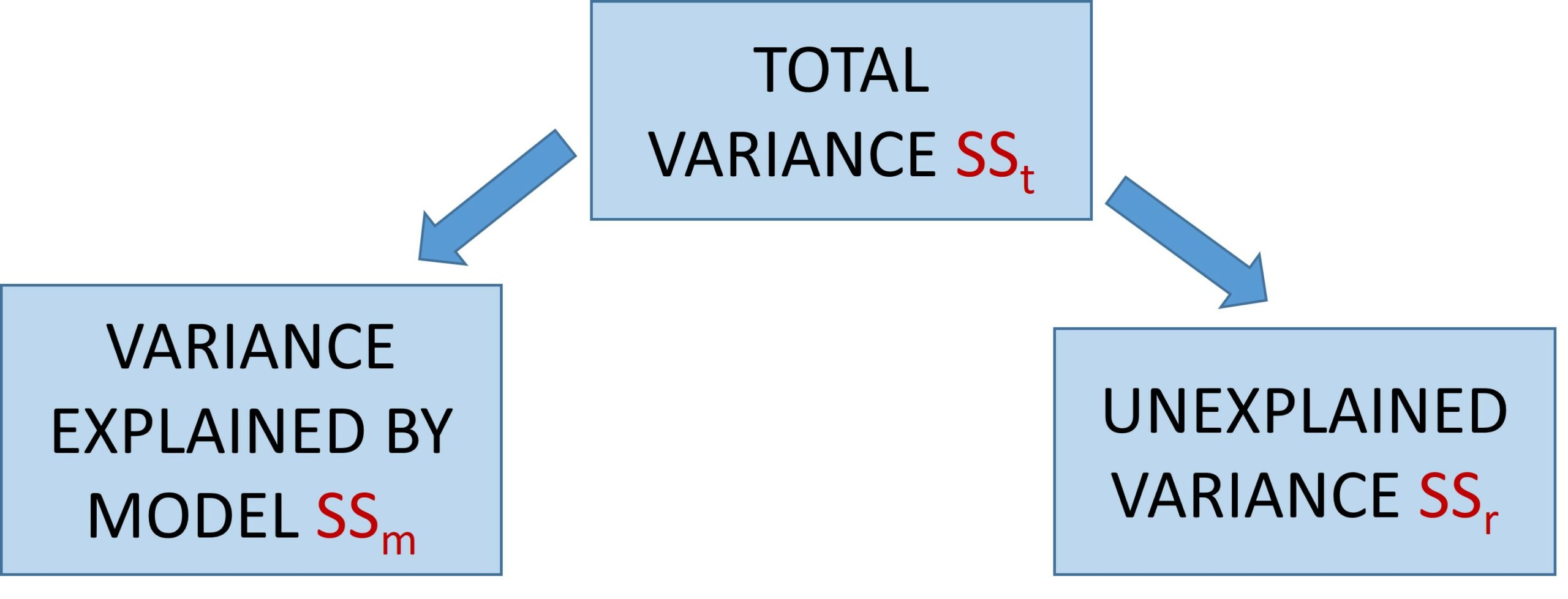
In other words, the one-way ANOVA, the variance is partitioned as follows:

The total variance, sum of squares total, SS_t, is an indication of how much all the scores in the experiment vary around the grand mean (i.e., the mean of all the scores). The model sum of squares, SS_m, sometimes reported as SS_b (between-groups sum of squares, for the one-way ANOVA) reflects how much the group means vary around the grand mean. And the residual sum of squares, SS_r, reflects how much participant scores vary around their own group means. So, SS_r is the amount of variability that is left over when we use the model (i.e., the group means) to predict scores, compared to when we just use the grand mean to predict scores. SS_r is the variability that we want to minimize. We want participants’ scores within each group to be as close as possible to their group mean, to make it easier to detect a difference between the groups.

To compute the one-way ANOVA, having completed the SS, we then compute mean square (MS, average variation):

We do this for both SS_m and SS_r. Next, we can compute F as follows: Now, one thing to keep in mind is that MS_m actually reflects variance not just due to the experiment but also it contains some error. There are going to be differences between your groups, not just due to the manipulation of the independent variable, but also due to extraneous variables. For example, we have different participants in each condition, and they are going to score slightly differently from each other even without the manipulation of the independent variable. What we are going to find out is whether the difference between the groups is larger than what we would expect if there were just extraneous variables at play. Note, on the other hand, that MS_r reflects only variability due to extraneous variables. So, when we compute F, if the null hypothesis is true (i.e., there is no effect of the independent variable on the dependent variable, i.e., no difference between the groups) then both MS_m and MS_r are just capturing variation due to extraneous variables (albeit calculated in different ways), and the F-value will be close to 1. On the other hand, if the null hypothesis is false, then MS_m will reflect both variability due to the manipulation of the independent variable and variability due to extraneous variables and so it should be larger than MS_r. As a result, F should be greater than 1 (note, this means that we only ever have a one-tailed test with ANOVA). At some point, F will be large enough that we will determine it is unlikely to be that large when the null hypothesis is true (when all means in the population are equal), and we claim that we have a significant effect.

You’ll sometimes see the formula for the one-way ANOVA as follows: where the “b” refers to “between-groups” (i.e., variation between-groups) and the “w” refers to “within-groups” (i.e., variation within groups).