39 Introduction to Regression
What is Regression?
Think back to the dataset we worked with in the previous chapter on correlation, where we looked at the association between a mum’s hours of sleep per night and her grumpiness, across 100 days. Imagine we would like to predict her grumpiness on any given day based on how many hours sleep she had. We can do this using regression. Regression goes beyond correlation in that it tells us not just the strength of the association between variables but also allows us to predict the value of one variable, the outcome, Y, from the value of another variable, the predictor, X. We do this by using the equation of a straight line (flash back to high school math, anyone?!). When we conduct regression, we describe the best fitting line that summarizes a linear relationship between our variables, and then we can use the equation for this line to predict scores.
Regression is a very useful tool, which can be extended into different contexts, such as when we have more than one predictor (multiple regression). Believe it or not ANOVA is actually the same thing as regression! You’ll see that when we compute regression, we can also compute F, just as we do in ANOVA! (But in regression we compute some other useful values about the relationship between our variables.) The actual connection is real – ANOVA and regression are based on the same fundamental statistics, but the details of that story are for another class.
The Straight Line
A linear regression model is basically a linear line, which many of us learned as y = mx + b, where y is our predicted outcome score, x is the IV, b is the intercept (the score in y when x = 0), and m is the slope (when you increase x-value by 1 unit, the y-value goes up by m units).
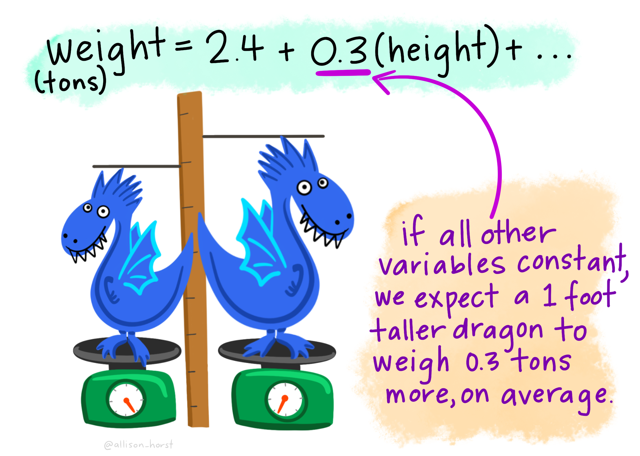
Let’s imagine we have a dataset of dragons with a single continuous predictor (height) and a continuous dependent variable (weight). (Note, we can also have categorial predictors in regression, but we shall touch on those later.) We want to use this dataset to be able to predict the weight of future dragons. First, let’s learn how to interpret the coefficients for our predictor variable.
“Artwork by @allison_horst” (CC BY 4.0)

This figure shows us that the weight of a dragon can be predicted by summing 2.4 plus 0.3 multiplied by the height of the dragon. This is an example of a regression equation, which describes the straight line that best fits the data when we plot X against Y.
In general terms, the regression line can be described as follows:
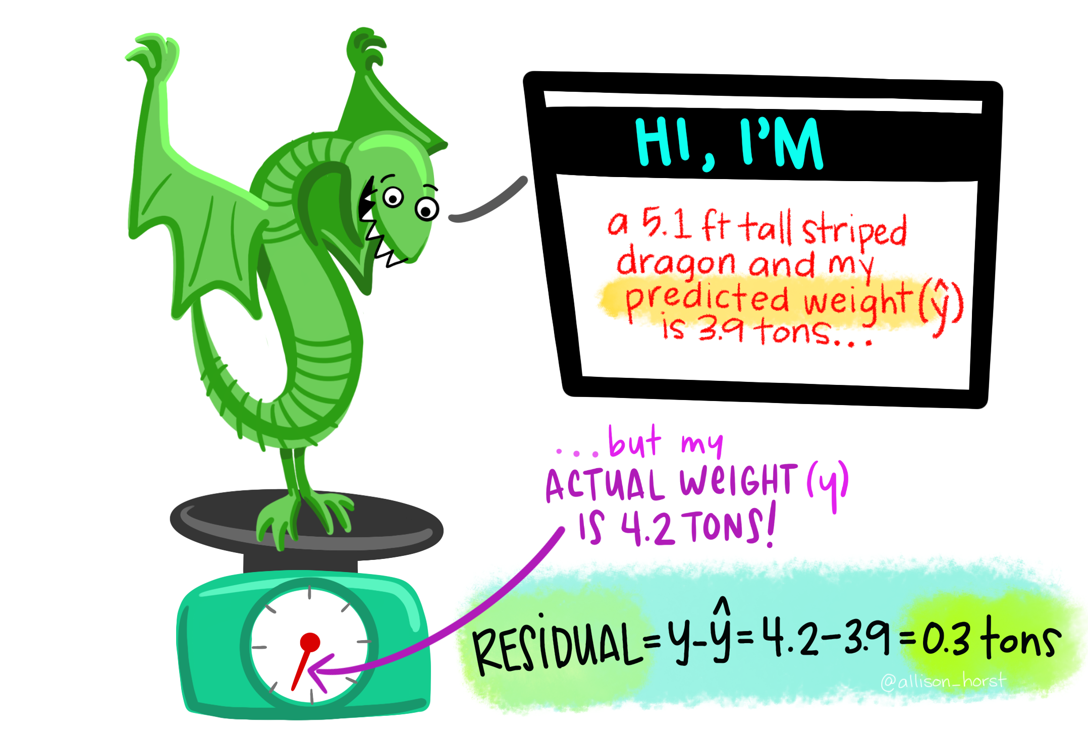
For any given datapoint, the errori term is called a residual. A residual is just the distance between the observed value for that entity and the predicted value, based on the regression model. See the dragon example below!
“Artwork by @allison_horst” (CC BY 4.0)

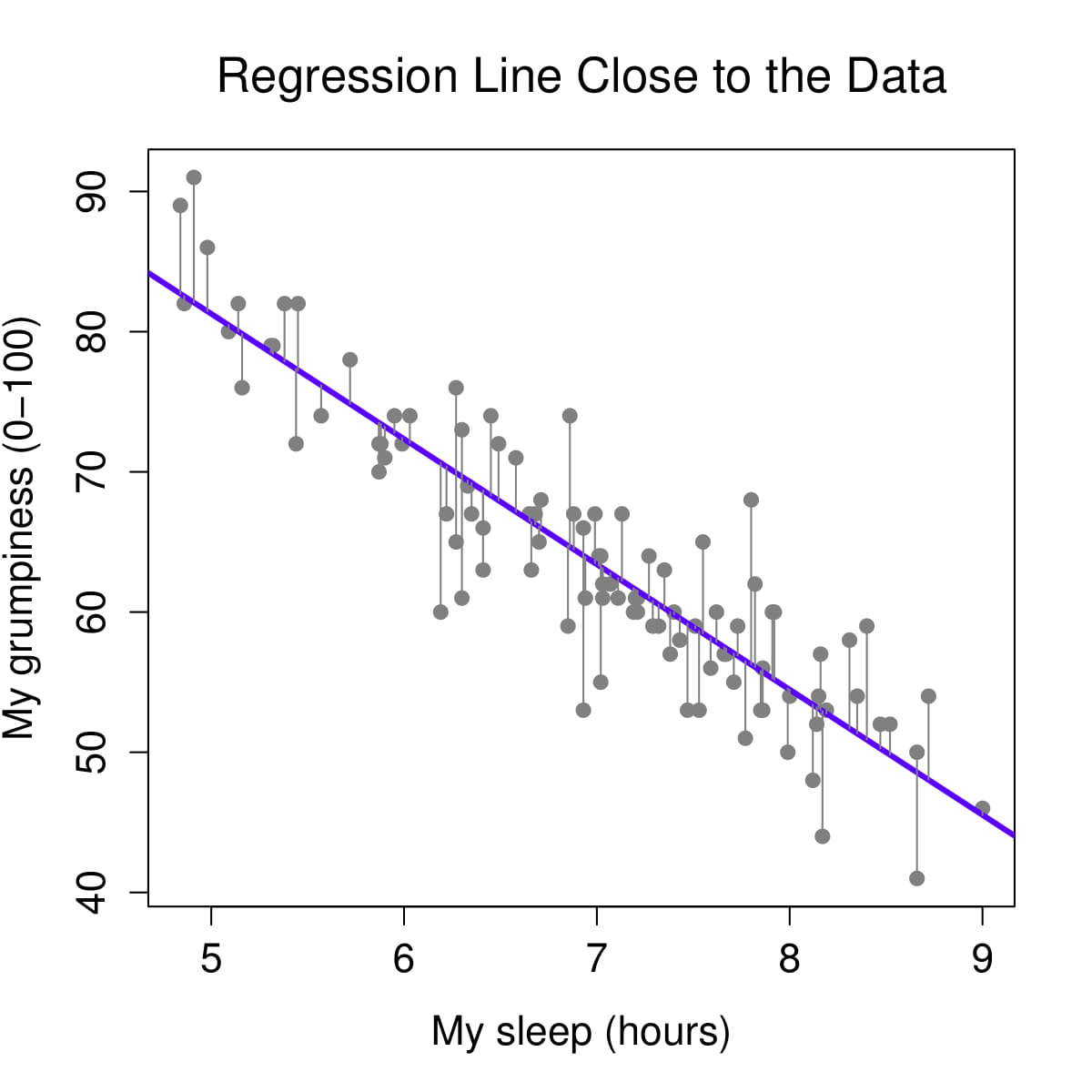
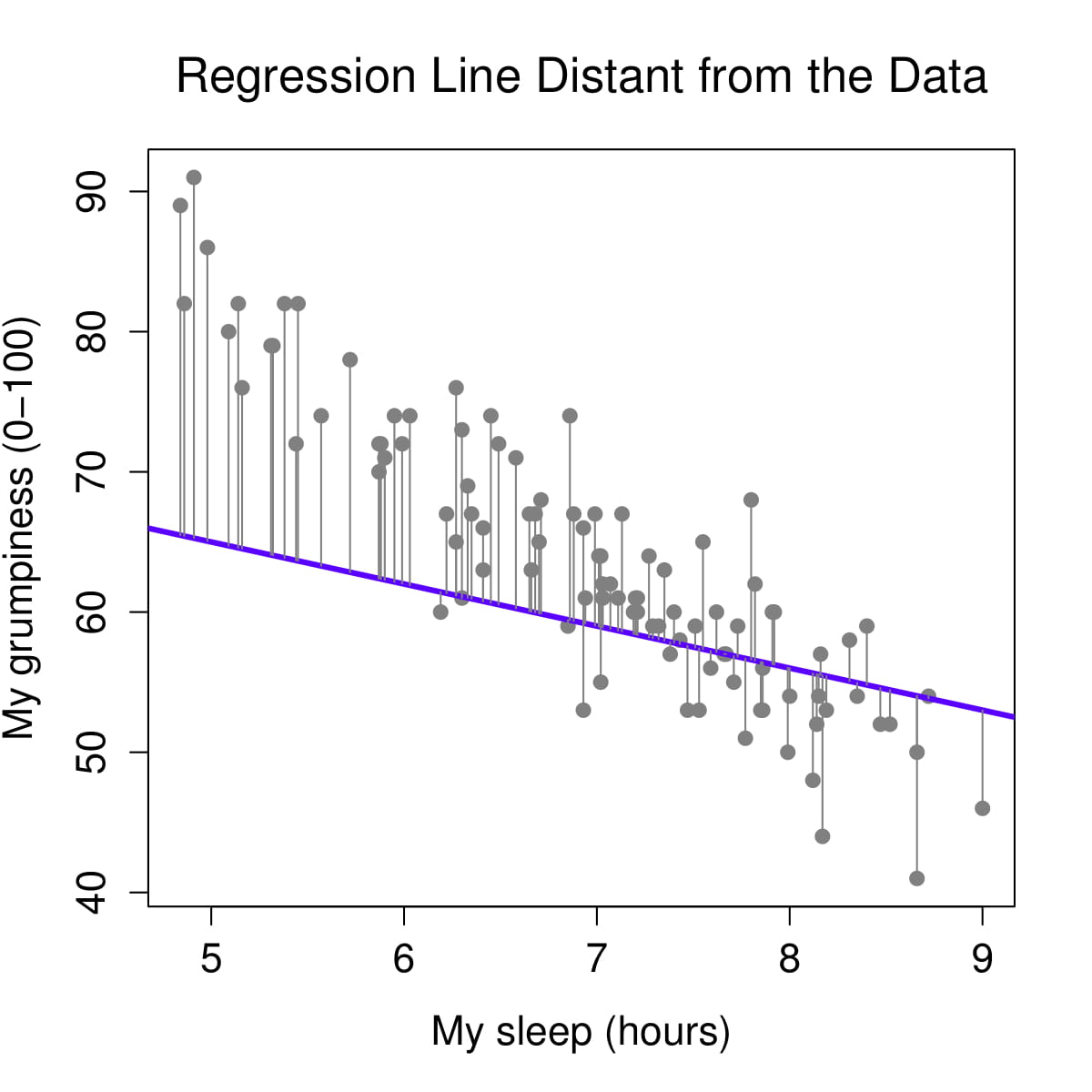
How are b0 and b1 determined? We determine our equation for the line from the scatterplot of scores by figuring out the line that fits closest to all data points. The regression line is the line that minimizes residuals – i.e., results in the smallest distance between the line and data points. Let’s visualize the regression line for how Dan’s sleepiness affect Dan’s grumpiness. Below on the left, we see the regression line (in purple) is very close to the data points and the residuals (the grey lines between the purple line and the data points) are smaller. On the right, we see the regression line is far from a lot of the data points and the residuals are larger.


The specific method to find this straight line is called the method of least squares. This is because the line obtained minimizes the sum of the squared residuals or the squared deviations from the line (fun fact: the method uses the squared residuals and not the raw residuals because the sums of the raw residuals will just be 0!). Fortunately, we do not have to sit there with a ruler and calculator and do this by hand – statistical software, including jamovi, does it for us!
In our graphs above, Total error = (observedi – modeli)2 . In other words, the total error in a model is just the sum of the (observed values minus the model values) squared. So the observed values are the datapoints, and the model values are given by the regression line. The difference between them is called a residual. This total error is the sum of the squared residuals, SSR, and so the regression line minimizes SSR.
