32 In Practice: Two-Way ANOVA
Let’s see how to conduct the two-way ANOVA in jamovi. We’ll start with a fully between-subjects design.
1. Look at the Data
Open data from your Data Library in “lsj-data.” Select and open “rtfm.” This data has two independent variables: attend (whether or not the student turned up to lectures) and reading (whether or not the student actually read the textbook). In both cases, 1 = they did and 0 = they did not. The dependent variable is their grade. There were eight participants in total. Note that the grade variable is currently set to be a nominal measure, but we should probably treat this as continuous, so go to Data, click on Setup, select the grade variable, and change the Measure type to Continuous.
Then you can obtain descriptive statistics (through Analyses, Exploration, Descriptives). When you obtain your descriptive statistics, note that you can either get them for the whole sample, or you can use Split by to get descriptives for each cell in your design. To use Split by, simply click and drag the attend variable and the reading variable to the Split by box. Note that we have a balanced design: there are 2 participants in each cell in our design.
Hypothesizing Main Effects and/or Interactions
We might hypothesize that both lecture attendance and reading will have a significant effect on students’ grades (i.e., two main effects), with improved grades for students who do versus do not attend/read. Would you predict an interaction? Before you read ahead, take a moment to think about whether you would predict an interaction and if you would, write it down.
Often, when learning about interactions, students might say that they would expect an interaction and describe it as follows: “students who both read and attend lectures will have the best grades and students who neither read nor attend lectures will have the worst grades.” Let’s come back to this statement in a moment. First, I would like you to sketch on a piece of paper what you would expect if there were just two main effects (improved grades for students who do versus do not attend class and improved grades for students who do versus do not read) and no interaction.
Now let’s look a bit more closely at this statement from above. There are three problems with this statement. The first is a general problem in that it describes how two particular cells in the design differ from the others, but it does not describe how the effect of one factor depends on or changes according to the level of the other factor. If we want to describe an interaction for this study, we would need to describe how the effect of attendance on grades is different according to whether or not students read. The second problem, which is related to the first, is that it’s not clear from that description what comparisons I am going to make when I want to break down the interaction – which groups will I compare with which? Will I just compare the attend+read group with the did not attend+did not read group? That would be a confounded comparison (which we have already discussed is not appropriate!).
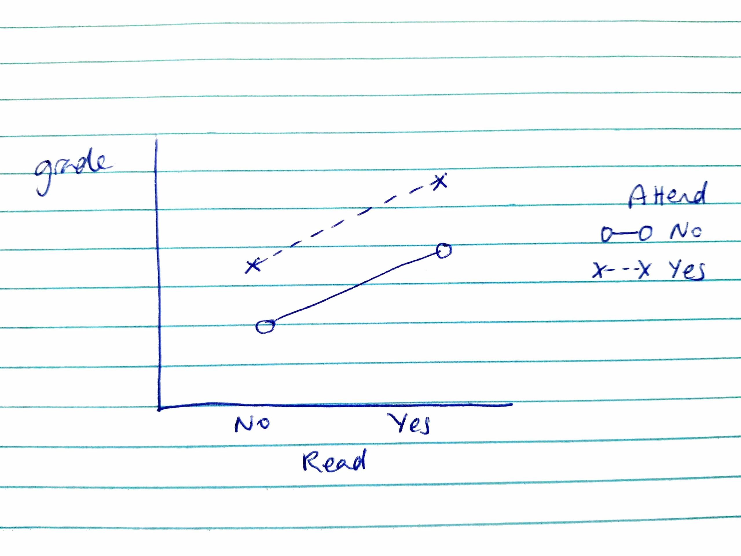
Now let’s take a look at the third problem. Go back to the sketch of two main effects that you drew a few minutes ago. Your sketch should look something like this (note, you could have Attend on the x-axis and Read as separate lines, and that would be fine, too!). Now, let’s look again at the statement from above: “students who both read and attend lectures will have the best grades and students who neither read nor attend lectures will have the worst grades.” Does the graph you drew capture the information provided in the statement? If you have a graph looks anything like mine, then it does! The point here is that the statement provided there does not describe an interaction. Rather, it describes the two main effects and shows that the consequences of reading and attending lectures are additive, not that the two independent variables interact.
So, if we did want to propose an interaction for these two variables, what might it look like and how would we describe it? Perhaps you expect that the effect of attendance on grades is greater for students who read than those who do not. Again, take a moment to sketch what this would look like. You should get something like this:
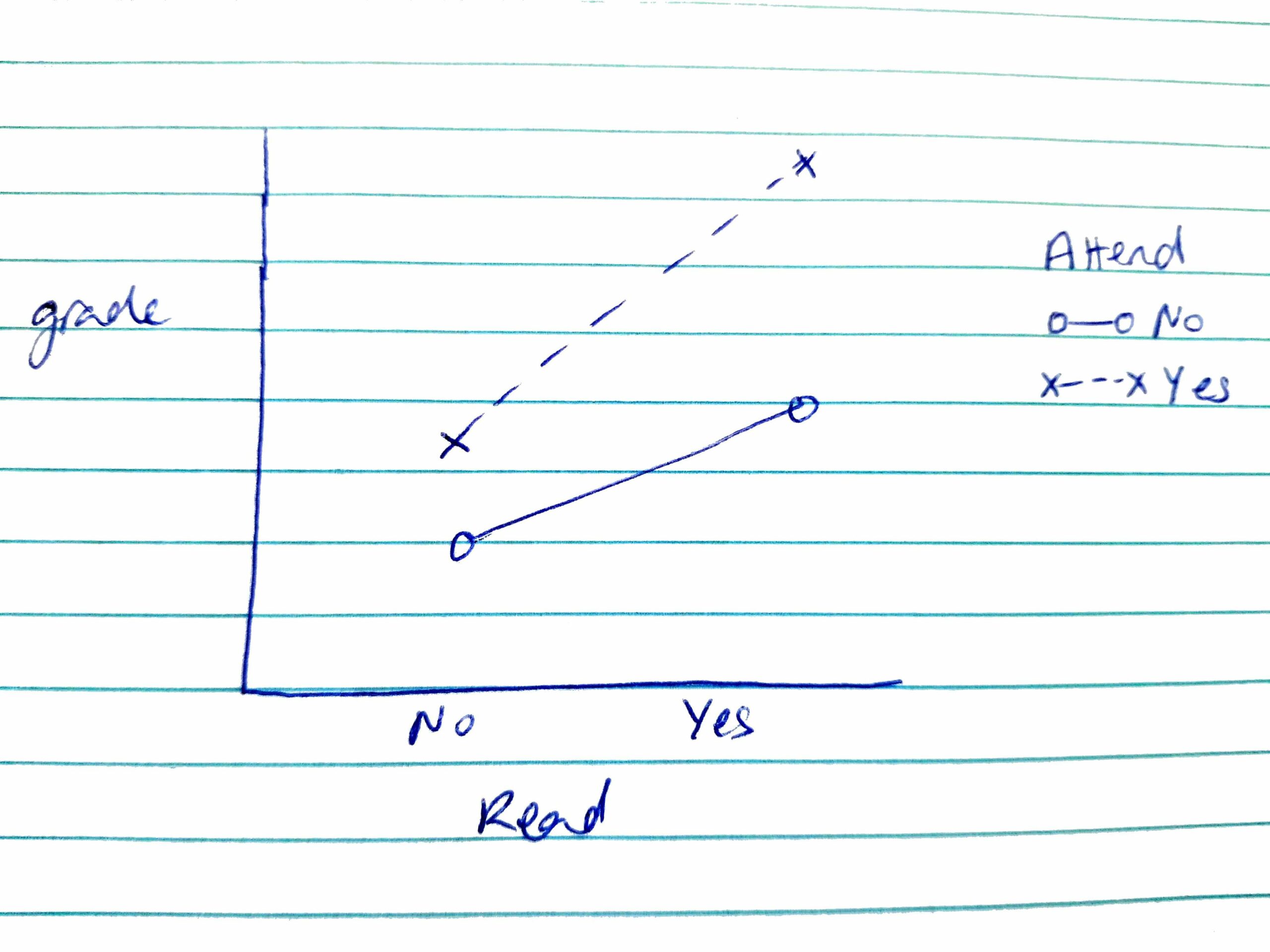
In this case, we might still have two significant main effects – it is the case that grades are higher for students who attend vs. do not attend, and for students who read vs. do not read. The interaction is an ordinal interaction (the lines do not cross), whereby the effect of reading on grades is greater for students who do attend vs. those who do not attend.
The main point of our digression here is to note that we should be very careful when we want to propose an interaction. Always sketch what you expect to find, and then describe what you see. When describing an interaction, remember to talk about how the effect of one factor changes according to which level(s) of the other factor you are looking at.
As we get ready to proceed with our example, let’s assume we are just predicting two main effects.
2. Check Assumptions
The assumptions for the two-way between-subjects ANOVA are the same as for the one-way ANOVA. Under the Analyses tab, select ANOVA, and then ANOVA. Move grade to the Dependent Variable box and attend and reading to the Fixed Factors box. You would then proceed to check for homogeneity of the variances and normality as we did for the one-way ANOVA, by selecting Homogeneity test, Normality test, and Q-Q Plot under the Assumption Checks drop-down menu. Remember the caveats about interpreting these tests: with small sample sizes they will not be significant, even if you have violated the assumption; with large samples they may be significant even with small deviations from normality/homogeneity of the variance. With this example dataset, we have a particularly small sample and so we would not usually proceed with this analyses because we cannot have any confidence that we have met the assumptions; however, for illustrative purposes, we are going to go ahead!
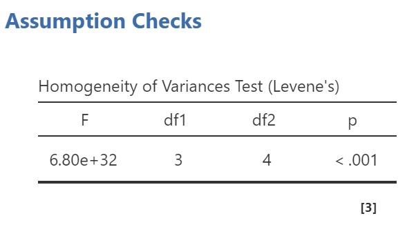 Surprisingly, Levene’s test for homogeneity of the variances is significant, in spite of the small sample size! So we have failed to meet that assumption. Unfortunately, we cannot perform Welch’s F-test when we have more than one factor, so we would note the failed assumption and move on.
Shapiro-Wilk’s test of normality was not significant and the Q-Q plot looks good, so we do not need to be concerned about deviations from normality (though again, remembering the caveat about small sample size in this particular instance).
3. Perform the Test
Next, we would perform the test. Make sure you select ω2 as your measure of effect size. Under Post Hoc Tests, there is no need to select post hoc tests for each factor, unless you have more than two levels of a factor. If you only have two levels, the post hoc tests will simply repeat your tests of the main effects. However, we can select the interaction term, attend * reading, and request a post hoc test for that. It will give us all the possible pairwise comparisons amongst the cells in our design. In our example, we did not predict an interaction (in cases where you do, see the box below about contrasts in factorial ANOVA), but we might wish to examine differences among cell means using the post hoc tests, in an exploratory fashion.
Contrasts in factorial ANOVA
Note that for the contrasts, jamovi will only provide comparisons within your main effects, not the interaction. Therefore, when you only have two levels for each factor, the contrast just gives you the same information as the main effect. If we had three levels of one of one of our factors, then we could select a contrast for that independent variable if we had some planned comparisons. For example, perhaps our attendance factor has three levels: attend live lecture, watch recorded lecture, do not attend or watch recorded lecture. In this case we might expect that grades are better for those who attend the live lecture than watch the recorded lecture and better for those who watch the recorded lecture than do not attend or watch the recorded lecture. In that case, we could request a Repeated contrast (see the section on Follow-up tests in chapter 6 for other types of contrasts). If you have planned comparisons and need contrasts to break down your interaction, see the sections on Interpreting interactions, earlier in this chapter.
We can use the Holm correction and request the effect size, Cohen’s d, for our post hoc tests. Under the Estimated Marginal Means menu, request plots and tables. Move attend to under Term 1, then click Add New Term and add reading under Term 2. Finally, click Add New Term again and move both attend and reading to under Term 3.
4. Interpret Results
Let’s look at the main results next.
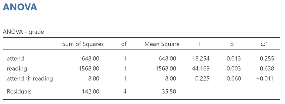
We got three lines of results in addition to the typical residuals (error). The first two rows are our main effects of attend and reading on grades. The p-values for both are statistically significant indicating attend affects grades and reading affects grades. However, it also added an interaction term, attend * reading, which is not statistically significant. This means we do not have an interaction between attend and reading on grades.
The results of the post hoc tests are as follows:
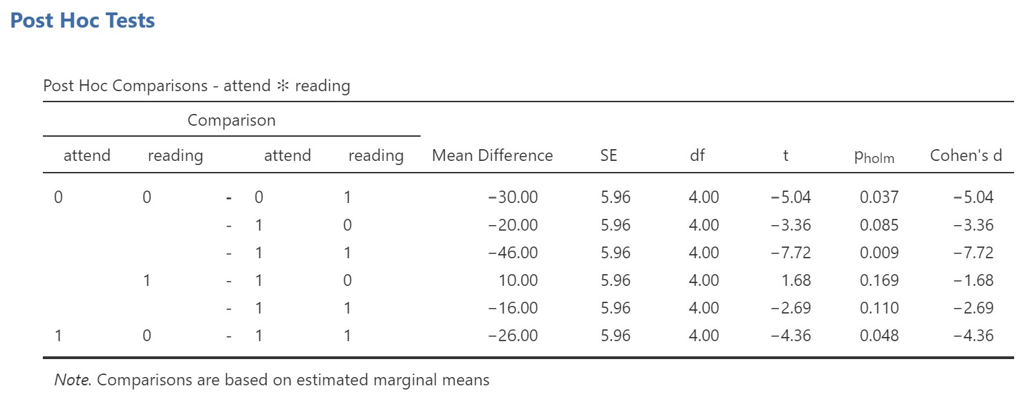
Because we do not have a significant interaction, the post hoc tests do not tell us anything more than the significant main effects. We already know from the ANOVA table that there is a main effect of both reading and attending, and so we would not look further at the post hoc tests. On the other hand, if the interaction had been significant, we could look at the post hoc tests to see where the differences in cell means lie. It can be pretty overwhelming to look at this table of post hoc results, so I recommend looking first at the plot of the marginal means.
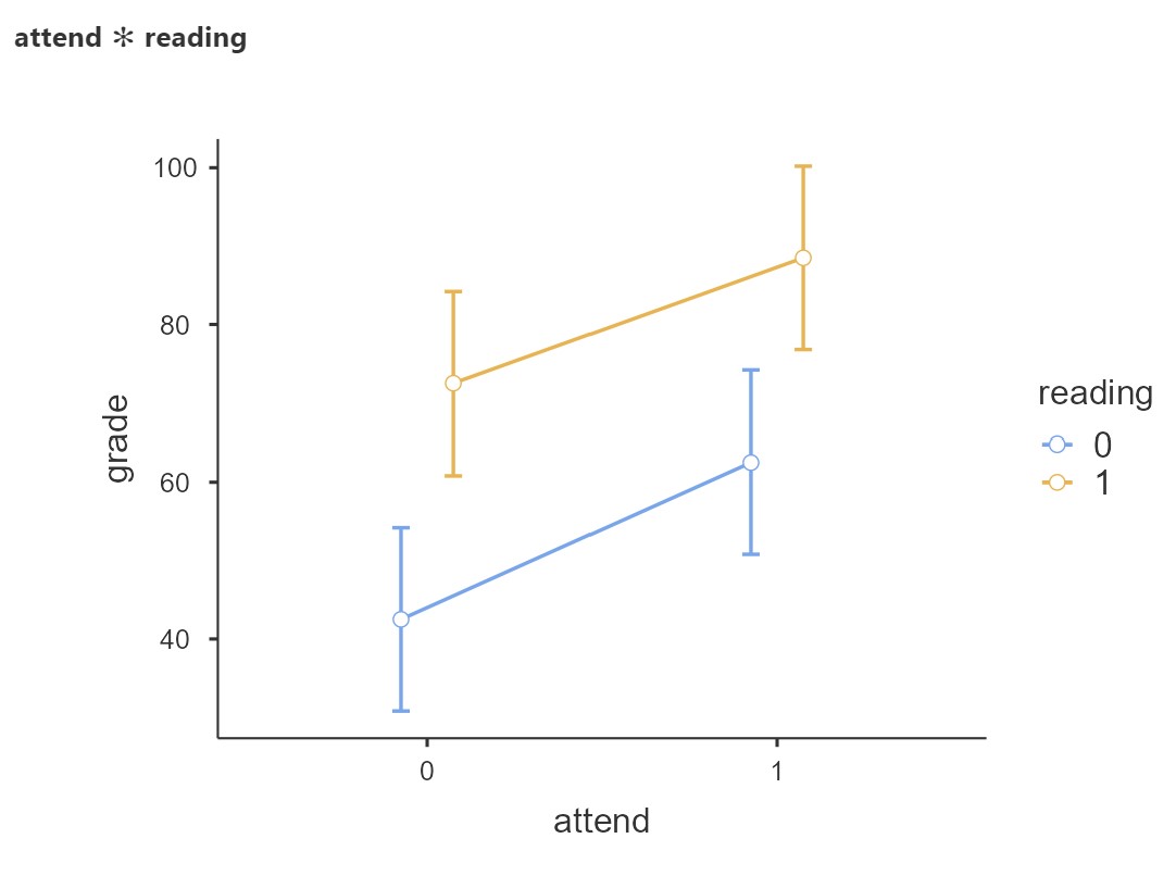
In class, we shall spend some time looking at one of these plots in an example where there is an interaction, so that we can explore how best to describe what is going on, using the results from the post hoc tests.
Write Up the Results in APA Style
We can then write up our results section. Note that we should describe the direction of any significant effects by stating which group scored higher than which, and reporting the relevant means from the Estimated Marginal Means tables.
I conducted a two-way between-subjects ANOVA to examine the effect of attendance and reading on student grades. Both attendance, F(1, 4) = 18.25, p = .013, = .26, and reading, F(1, 4) = 44.17, p = .003, = .64, affected student grades; there was no significant interaction between attendance and reading, F(1, 4) = 8.00, p = .660. Students who attended lectures (M = 75.50, SE = 2.98) had higher grades than students who did not (M = 57.50, SE = 2.98). Students who read (M = 80.50, SE = 2.98) had higher grades than students who did not (M = 52.50, SE = 2.98).
In this case, we did not have a significant interaction. But what if the interaction term was significant? Then, we could report the post hoc tests that best help us support the description of the interaction we obtained when following the steps to describing an interaction (to be outlined and practised in class). Of course, if we had planned comparisons, we would report only the comparisons that we had planned a priori. Therefore, when planning an experiment where you will use factorial ANOVA, it is a good idea to think very carefully about what kind of interaction you expect to see – sketch a graph of the pattern of results you expect to see in order to decide what planned comparisons you wish to make.
