18 In Practice: t-Tests
Let’s take a look at how to run the independent samples and dependent samples t-tests using jamovi.
Remember our four steps to data analysis:
- Look at the data
- Check assumptions
- Perform the test
- Interpret results
Please install the lsj-data module by clicking on the plus sign in the top right hand corner of the jamovi window. Once you have installed it, close jamovi and re-open it. When you go to Open and select Data Library, you’ll see a new folder called “learning statistics with jamovi.” In that folder, you’ll find several example datasets that we shall use in the remainder of this book.
Independent Samples t-Test
For now, open “Harpo.” This dataset is hypothetical data of 33 students taking Dr. Harpo’s statistics lectures. We have two tutors for the class, Anastasia (n = 15) and Bernadette (n = 18). Our research question is “Which tutor results in better student grades?”
1. Look at the Data
To conduct the independent t-test, we first need to ensure our data is set-up properly in our dataset. This requires having two columns: one with our continuous dependent variable and one indicating which group the participant is in. Each row is a unique participant or unit of analysis.
Below are the first ten rows of our data from the Harpo dataset.
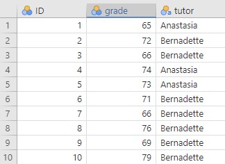 In this dataset, what is the independent variable and what are the levels? What is the dependent variable?
Notice that the variable “grade” is set up as a nominal variable, but we should change this to continuous. Once we have done so, we should look at our data using descriptive statistics. As you learned before, select Exploration and Descriptives. They are shown below. You’ll see that I split the data by tutor. I left the default settings for the statistics and also requested Histogram and Density under Plots.
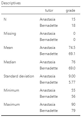
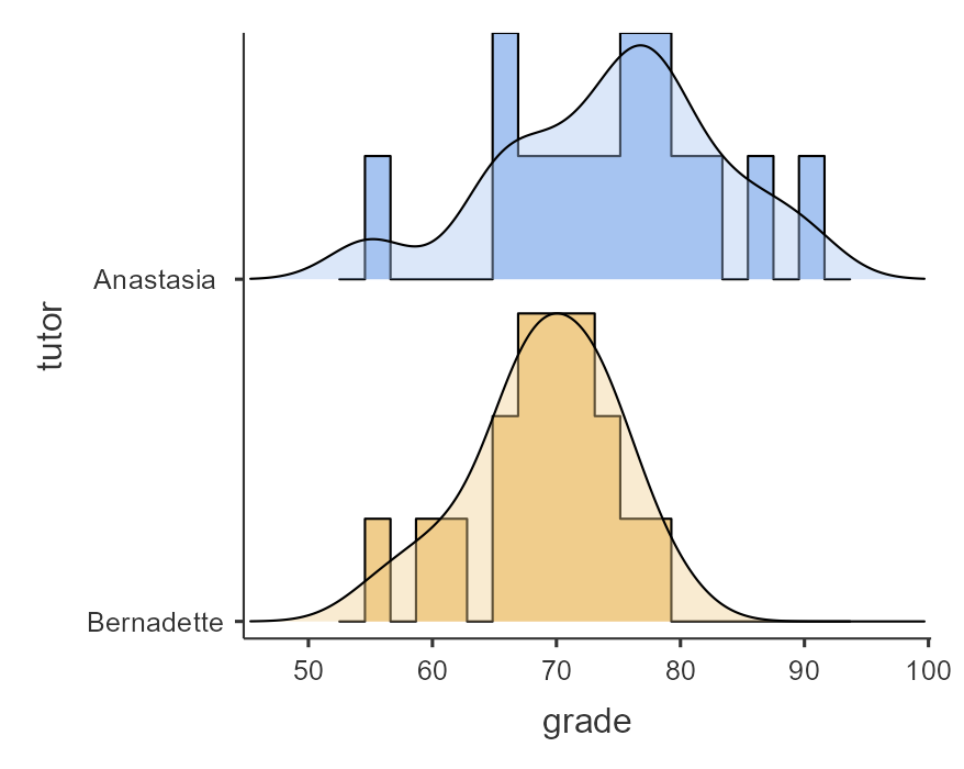
Our overall data consists of 33 cases. The minimum and maximum values look plausible; theoretically, student grades should range from 0-100. Lastly, the distribution of data looks roughly normally distributed. Before we proceed with our analyses, we should look a bit more closely at our assumptions.
2. Check the Assumptions
The dependent variable seems to be ratio data (grade) and let’s assume that whoever collected these data is certain that scores are independent (no students attended both Anastasia’s and Bernadette’s tutorial sessions!). What about normality and homogeneity of the variances?
Check Normality
We can check normality by adding a request for Normality test and Q-Q plot under the Assumption Checks when we request the independent samples t-test: go to Analyses, T-Tests, and then Independent samples T-Test. Select the grade variables in the Variables box, and put the tutor variable in the Grouping variable box. Under Statistics select the Q-Q plot and Normality test.
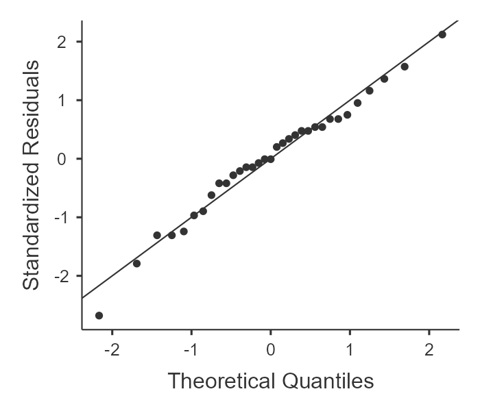 The Q-Q plot, shown on the right, is created as follows: each observation from the dataset is plotted as s single dot, where the x coordinate is the theoretical quantile that the observation should fall in if the data were normally distributed (with mean and variance estimated from the sample), and the y co-ordinate is the actual quantile of the data within the sample. If the data are normal, the dots should form a straight line. Ours looks pretty good – and what we see is in alignment with what we would expect given the visual inspection of the histograms above.
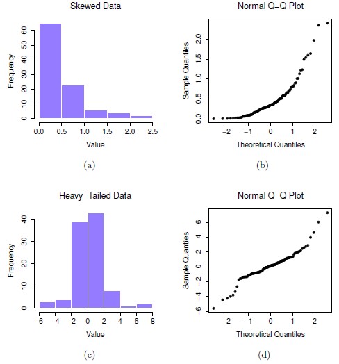
On the other hand, the examples on the left show data that are not normally distributed. (a) and (b) are the histogram and Q-Q plot for positively skewed data and (c) and (d) show the histogram and Q-Q plot for data with heavy tails (i.e., high kurtosis). In each case, you can see that the histogram does not show a nice, normal shape, and dots on the Q-Q plot do not fall close to a straight line.
Another way to assess normality is by examining the results of the Shapiro-Wilk statistic. The Shapiro-Wilk statistic is produced by your having checked the Normality test box (note, you can also obtain both this test and the Q-Q plot in the Descriptives when you initially explore your data).
The Shapiro-Wilk test assesses whether the data deviate significantly from normality. We interpret it the same way we would any other inferential test. If p < .05 then the data deviate significantly from normality. In our case, with the grade variable from the Harpo dataset, the value for the Shapiro-Wilk statistic W = 0.98, and p < .827. Therefore, it is not significant and we would conclude that the data do not deviate significantly from normality.
However, in reality, it is a bit more complicated than that. First, many would argue that the assumption is not that the data themselves should be normally distributed, but that the sampling distribution should be normally distributed. You may recall, for example that the sampling distribution of the means is always normal, regardless of the shape of the distribution of the underlying raw scores, as long as the sample is large enough (at least N = 30; you might remember this from central limit theorem and I’ll show you a demo of this in class!).
In addition, there’s a caveat to interpreting the Shapiro-Wilk test. As you’ll recall from earlier in this book, sometimes we do not have enough power to detect something that actually exists in the population, and we can make a type 2 error as a result. You might also remember that sample size, effect size, alpha, and power are all interrelated and that a small sample size yields lower power than a large sample size (all other things being equal). What this means is that with small sample sizes, Shapiro-Wilk may not be significant even with relatively large deviations from normality. And, it is with small sample sizes that central limit theorem does not hold. In other words, with small sample sizes, the Shapiro-Wilk test might tell you that the data are normally distributed (because you do not have enough power to detect non-normality) and you cannot safely assume that the sampling distribution will be normally distributed. Thus, there is a risk that you are unknowingly violating the assumption of normality.
Fortunately, there is a solution. If you are concerned about normality, especially with a small sample, you can use what is called a “robust t-test.” A robust test is a version of the test that is less impacted by violations or normality. For the t-test, in jamovi, you can download the Walrus package and use the robust t-test within that package (there’s a robust test for independent samples and for dependent samples; use the default trim proportion of 0.2). Another alternative is to use the Mann-Whitney U test (this one is available with the regular jamovi t-tests options).
Checking Homogeneity of the Variances
The assumption of homogeneity of the variances is that the variances (in the population) are homogenous (i.e., the same). If they are not close enough in our sample, then we cannot trust the result of the t-test. You can easily test for homogeneity of the variances in jamovi: when you select your t-test, you can request the Homogeneity test (again, under Assumption Checks). This will produce Levene’s test for equality of variances. This test does exactly what the name suggests: it tests whether the variances in the two groups are significantly different from each other. If the p-value from this test is < .05, then the variances are significantly different. However, the same caveat applies here as to our interpretation of the p-value for the Shapiro-Wilk test: if our sample size is small, power will be low, and we will not be able to detect differences between the variances even when they are quite large. At the other end of the spectrum, with large samples, the test may be significant even when there is only a small difference in the variances. It is for this reason that many researchers now recommend using Welch’s t-test instead of the Student’s t-test (Student’s is the standard one that you probably learned about in your lower level stats class). Welch’s t-test does not make the same assumption of homogeneity of the variance. Fortunately, Welch’s t-test is easily available to us in jamovi: you will see it as an option under the Student’s test.
In our Harpo dataset that we are working with, Levene’s test for homogeneity of the variances shows that p = .125 (i.e., not significant). This suggests that the variances of the grades of the two groups (i.e., students who had Anastasia as a tutor vs. those who had Bernadette as a tutor) are not significantly different from each other. However, as discussed above, with small samples, we cannot trust Levene’s test. We should probably use Welch’s t-test.
3. Perform the Test
“At last!” I hear you sigh. Let’s imagine you had proposed a two-tailed hypothesis: that there will be a difference in grades for Anastasia’s and Bernadette’s students. Now you can do your inferential test and answer the question: did Anastasia’s students and Bernadette’s students have significantly different grades?
Do not forget the outcome of the assumption checks. We talked about how, given the sample size, we should be cautious about interpreting the Shapiro-Wilk test and Levene’s test. You might be wondering if you should do the Robust test or Welch’s t-test in this situation. A glance at the histogram showing the distribution of scores suggested that the raw scores themselves are somewhat normal. Thus, in this case, I would recommend we go with Welch’s t-test. Let’s also get the Student’s t-test and we can see how the results compare.
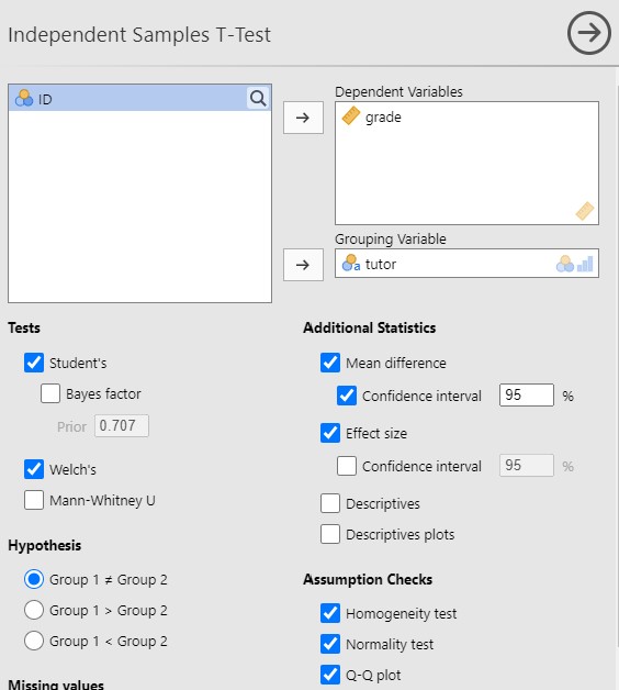
In the Analyses tab, select T-Tests and Independent Samples T-Test. Ensure that you move the grade variable over to the Dependent Variables box, and the tutor Variable over to the Grouping Variable box.
You’ll note on the right that I’ve selected both Student’s and Welch’s. In addition, I have requested the Mean difference and Confidence interval, as well as Effect size. If you wish, you can get Descriptive statistics and plots again.
Under Hypothesis, I have specified that I am interested in a two-tailed test – I am simply predicting that there is a difference between the two groups, rather than the direction of the difference.
4. Interpret Results
Let’s look at the output, below:

If we look at the Student’s t-test result, our p-value is less than our alpha value of .05, a statistically significant result. Like most of the statistics we’ll come across, the larger the t-statistic (or F-statistic, or chi-square statistic…), the smaller the p-value will be.
However, remember that we were a bit concerned about assuming homogeneity of the variances, given the small sample size? Therefore, let’s look at the Welch’s t-test result instead. Here you will see that the p-value is .054. This is not statistically significant. Remember the small sample size? This is rather concerning and our study would be underpowered. In fact, if I go into the jpower module in jamovi, I find that we have only 28% power to detect a medium effect size, d = .50 (see below) and 60% power to detect a large effect, d = .80!

This study really needed to have a larger sample size (and the researcher should have determined, a priori, what the effect size of interest was, and what sample size would be required to detect that effect.
Write Up the Results in APA Format
Finally, we can write up the results. We should always include the following information:
- Description of your research question and/or hypotheses and the test used to assess it.
- Description of your data – in this case means and standard deviations for each group. If you fail to meet assumptions, you should specify that and describe what test you chose to perform as a result.
- The results of the inferential test, including what test was performed, the test value and degrees of freedom, p-value, and confidence intervals (in this case around the difference between the means). If the effect is significant, then also report effect size.
- Interpretation of the results, including any other information as needed.
We can write it up something like this:
I used Welch’s independent samples t-test to assess whether there was a difference in student grades between Anastasia’s and Bernadette’s classes. Anastasia’s students (M = 74.5, SD = 9.00) had did not have significantly higher grades than Bernadette’s students (M = 69.1, SD = 5.77), t(23) = 2.03, p = .054, Mdiff = 5.48, 95% CI [-0.09, 11.00].
(Note that I did not report d, the effect size, because the result was not significant.)
A note about positive and negative t values
Students often worry about positive or negative t-statistic values and are unsure how to interpret it. Positive or negative t-statistic values simply occur based on which group is listed first. Our t-statistic above is positive because we tested the difference between Anastasia’s class (M = 74.53) versus Bernadette’s class (M = 69.06) and so Anastasia – Bernadette is a mean difference of 5.48.
However, if our classes were reversed, our mean difference would -5.48 and our t-statistic would be -2.12.
All that is to say, your positive or negative t-statistic is arbitrary and is just a function of which group is listed first, which is also arbitrary. So do not fret!
One last note: this positive or negative t-statistic is only relevant for the t-test. You will not get negative values for the F-statistic or chi-square tests!
Dependent Samples t-Test
We are going to work with the chico dataset in the lsj-data Data Library. Open the dataset now.
1. Look at the Data
This dataset is is hypothetical data from Dr. Chico’s class in which students took two tests: one early in the semester and one later in the semester. Dr. Chico thinks that the first test is a “wake up call” for students. When they realise how hard her class really is, they’ll work harder for the second test and get a better mark. Is she right?
Data Set-Up
To conduct the dependent t-test, we first need to ensure our data is set-up properly in our dataset. This requires having two columns: one is our dependent variable score for the participant in one category and the other column is our dependent variable score for the participant in the other category. Each row is a unique participant or unit of analysis. The first few rows of your data should look like this:
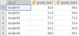 In this dataset, what is your independent variable? What is your dependent variable?
Describe the Data
Once we confirm our data is setup correctly in jamovi, we should look at our data using descriptive statistics and graphs. To get descriptive statistics, go to Exploration, then Descriptives. Move the two dependent scores (grade_test1 and grade_test2) over to the Variables box.
Our descriptive statistics are shown below.
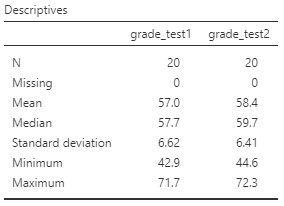 Our overall data consists of 20 cases (students) and the average grade is 56.98 (SD = 6.62) at the first test and 58.38 (SD = 6.41) at the second test. We have no missing cases, and our minimum and maximum values look accurate; theoretically, student grades should range from 0-100. Lastly, the distribution of data looks fairly normally distributed, although I’m personally a little worried about our small sample size. Before we can proceed with our analyses, we’ll need to check our assumptions.
Let’s assume that Dr. Chico thinks that the first test is a “wake up call” for students. When they realise how hard her class really is, they’ll work harder for the second test and get a better mark. That suggests Dr. Chico thinks students will have better scores on the second test compared to the first test, so it is a directional prediction, which calls for a one-tailed test.
2: Check Assumptions
As a parametric test, the dependent t-test has the same assumptions as other parametric tests (minus homogeneity of variance because we are dealing with the same people across categories):
- The differences in scores in the dependent variable are normally distributed
- The dependent variable is interval or ratio (i.e., continuous)
- Scores are independent across participants
We cannot test the second and third assumptions; rather, those are based on knowing your data and research design.
However, we can and should test for the first assumption. Fortunately, the dependent samples t-test in jamovi has two check boxes under “Assumption Checks” that lets us test normality. The same caveat applies as for checking normality for the independent samples t-test.
One thing to keep in mind in all statistical software is that we often check assumptions simultaneously to performing the statistical test. However, we should always check assumptions first before looking at and interpreting our results. Therefore, whereas the instructions for performing the test are below, we discuss checking assumptions here first to help ingrain the importance of always checking assumptions for interpreting results.
Testing Normality
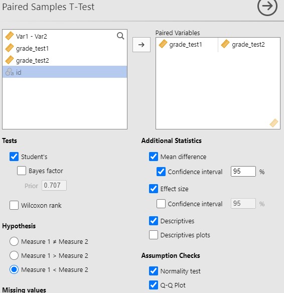
Notice how our dependent variable is really the difference in scores, and therefore that is what we are testing for normality. The easiest way to do this is by selecting the Paired Samples T-Test (under T-Tests) and entering your variables as described in step 3 below. Under Assumption Checks, you can then select Normality and Q-Q Plot.
If you want to test normality via the Descriptive options, there’s an extra step to do. First, you need to calculate a new variable that is the difference in scores. Go to Compute and enter into the formulate box Var1 - Var2 (in this case, grade_test1-grade_test2). Rename it to something meaningful to you. Then you are going to use that variable to test for normality. Select Exploration and Descriptives and choose the new variable that you just created. Select the Shapiro-Wilk test and, under Plots, the Q-Q plot, as well as looking at the density/histogram plot . The Shapiro-Wilk test was not statistically significant (W = .97, p = .678), suggesting the data are normally distributed – but remember the caveat about interpreting this result when we have a small sample size! Furthermore, the lines are fairly close to the diagonal line in the Q-Q plot (although it’s a bit hard to tell because our sample size is small). The histogram shows a roughly normal distribution. I would be hesitant to assume normality because the sample size is so small (N = 20) and I would recommend using the Wilcoxon rank test (the non-parametric equivalent to the dependent samples t-test – more on that later), but for illustrative purposes, let’s run the dependent samples t-test anyway.
3. Perform the Test
4. Interpret Results

Write up the Results in APA Format
Finally, we can write up the results:
I conducted a dependent samples t-test to assess whether students performed better on the second test compared to the first test. The students performed better on the second test (M = 58.4, SD = 6.41) than they did on the first test (M = 57.0, SD = 6.62), t(19) = 6.48, p < .001, d = 1.45, Mdiff = -1.40, 95% CI [-Inf, -1.03].
What if the result of our inferential test is not significant? In this case, we would report that there was no significant difference between performance on the first and the second test, providing the same statistical values as above, except that we would not need to report the measure of effect size.
