35 Analysis of Covariance
When Do We Use ANCOVA?
We use analysis of covariance (ANCOVA) when we want to test for differences among group means, but we suspect that a measured extraneous variable also affects the dependent variable. ANCOVA allows us to test the effect of the independent variable on the dependent variable, while controlling for the relationship between the extraneous variable and the dependent variable. The benefit of using this test is that it controls for unsystematic variation and so reduces error variance.
Let’s look at an example from the lsj-data Data Library. Open the dataset called ancova. This data is fictional data from a health psychologist who was interested in the effect of transportation used to commute (1 = driving, 2 = cycling) and stress (1 = high, 2 = low) on happiness levels, with age as a covariate. (This is actually a 2 x 2 independent factorial design with a covariate!) For the purposes of introducing ANCOVA, let’s keep it simple and just focus on the commute independent variable, with age as the covariate.
1. Look at the Data
I’ll assume by now that you know how to look at your descriptive statistics! I recommend first changing the age variable to continuous (it is not nominal!). You should also obtain the descriptive statistics for the covariate. I have copied the descriptive statistics below, split by commute – it will be interesting to compare these to the marginal means, later!
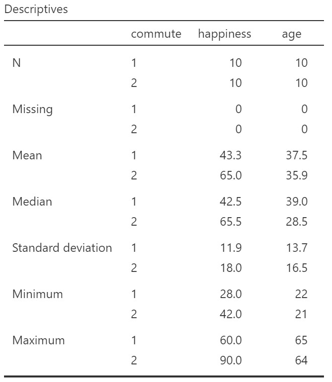
Our hypothesis is that there is a significant effect of transportation used to commute on happiness, when controlling for age. Specifically, we might predict that people who ride are happier than people who drive.
2. Check Assumptions
ANCOVA has the same assumptions as the one-way ANOVA (normal distribution, homogeneity of the variances, interval or ratio data, scores are independent between groups) and there are two additional assumptions we need to check. Let’s focus on those here.
1. No Significant Effect of IV on Covariate
Check to see if there is a significant effect of the independent variable (commute) on the covariate (age). Run an ANOVA with commute as the Fixed Factor and age as the Dependent Variable in jamovi. There should be no significant effect! We can see that there is no significant effect of commute on age, so we are safe to proceed.

2. Homogeneity of Regression Slopes
The second additional assumption is that the relationship between the covariate and the dependent variable is similar for all levels of the independent variable (homogeneity of regression slopes). In other words, the relationship between age and happiness levels should be similar for the drivers and the cyclists. There are two ways to investigate this question. First, we can produce a scatterplot showing the relationship between age and happiness for drivers and for cyclists – i.e., let’s plot the regression slopes to see if they look the same (homogeneous) or not.
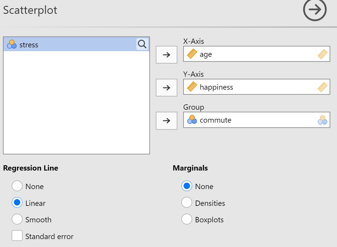
In jamovi, select Exploration and Scatterplot (from the scatr module – if you did not already install this, you will need to do so). Move age to the X-Axis, happiness to the Y-Axis, and commute to the Group. Select Linear for the regression line. The regression line will show the best fit line through the points on the scatterplot (more on regression lines in a later chapter).
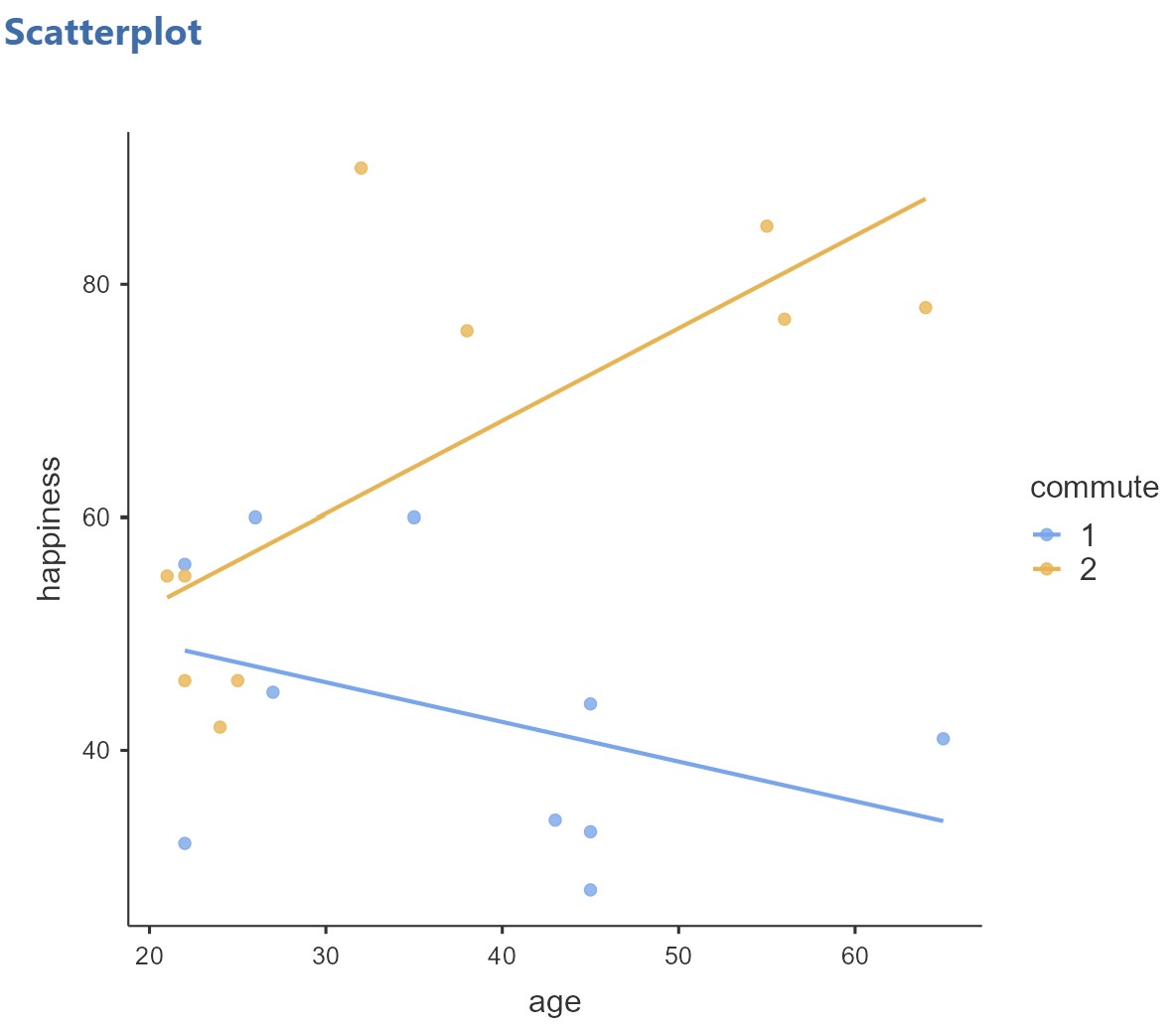
In the scatterplot above, the blue dots and line represent the drivers and the orange dots and line represent the cyclists. It looks like for the drivers, happiness decreases with age, and for the cyclists, happiness increases with age. We may have violated the assumption, but to check whether this difference in the regression slopes is significant, we need to go further.
In jamovi, select the ANOVA button under Analyses, and then select ANCOVA. Move happiness to the Dependent Variable box, commute to the Fixed Factors box, and age to the Covariates box. This is how we would normally set up our ANCOVA. To check homogeneity of the regression slopes, now go into the Model drop-down menu to add an interaction term between the covariate and the independent variable. To do this, hold down the Shift key on your keyboard and click on both commute and age. Then click on the little arrow with the drop-down menu and select Interaction. Commute * age will then show in the box under Model Terms.
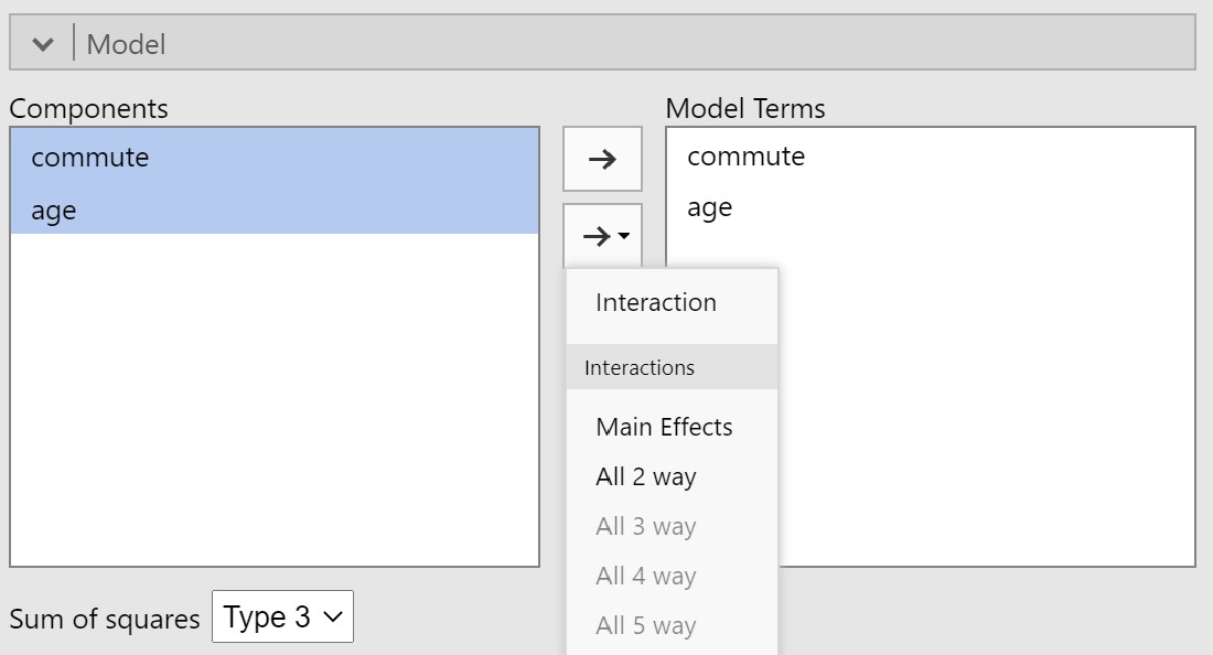
We can now examine the ANCOVA table to see if there was a significant interaction between commute and age in the effects on happiness.
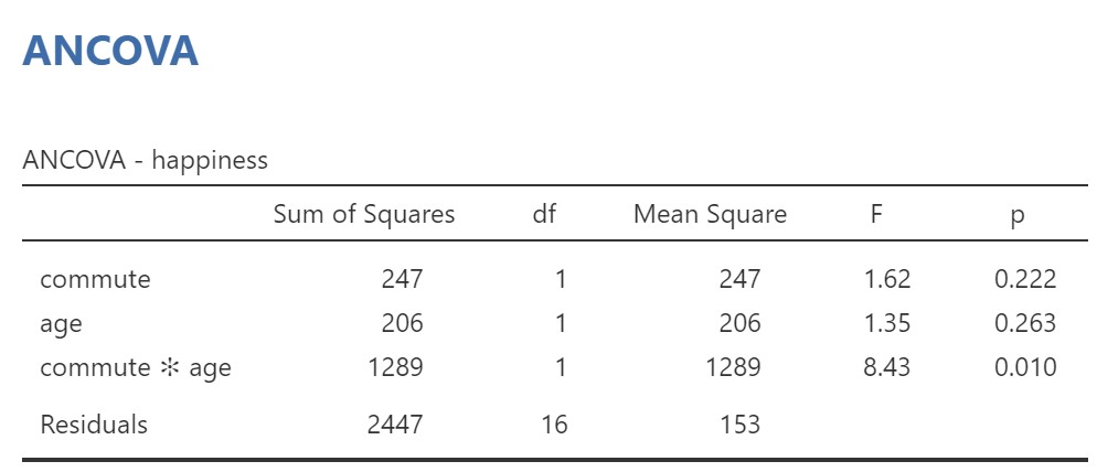
When we look at third row of the table above (commute * age), p = .010, which means there is a significant interaction between commute and age and the assumption of homoegeneity of the regression slopes has been violated (i.e., the regression slopes are not homogenous, they are heterogenous).
Note that sometimes heterogeneity of the regression slopes may be interesting or expected – perhaps we even expect that cyclists, but not drivers, should get happier with age! If so, then we need to go to another kind of statistical model, called the multilevel model, but that is beyond the scope of this book. Having violated the assumption of homogeneity of the regression slopes, we should also go to a multilevel model, but for illustrative purposes, let’s proceed with our ANCOVA.
3. Perform the Test
To perform the ANCOVA, we can start a fresh analysis in jamovi. Select ANCOVA under the ANOVA analysis menu and again, Move happiness to the Dependent Variable box, commute to the Fixed Factors box, and age to the Covariates box. Select ω2 for effect size and this time do not make any edits to the model.
There is no need to run contrasts or post hoc tests because we only have two levels of our factor (but if we had three or more levels, we would likely choose to run one of them according to whether or not we had specific predictions about differences among levels of the independent variable.
Under Estimated Marginal Means, move the commute variable to the Term 1 box, select both plots and tables and unselect Equal cell weights.
4. Interpret Results
The results are shown below.
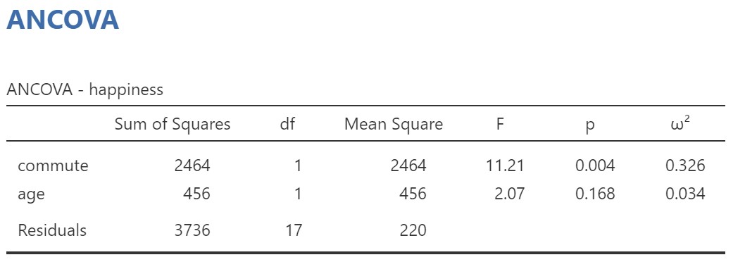
The ANCOVA table shows us that the effect of commute on happiness is statistically significant. The relationship between age and happiness is not significant overall, but this does not matter – what we are interested in is whether commute affects happiness while controlling for the relationship between age and happiness. Even if age and happiness are not significantly associated, controlling for age will still help to reduce error variance with the groups in our experiment and increase power in our design.
In some situations, the effect of the independent variable on the dependent variable is no longer significant when the covariate is removed from the analysis. Let’s check if that is the case. We can re-run the analysis but just remove the covariate. When we do that, we get the following result:

Comparing this with the table above we can see that the F-value is slightly smaller and the p-value therefore slightly larger. Thus, including the covariate in the analysis did reduce error variance!
Let’s look at the table of marginal means:
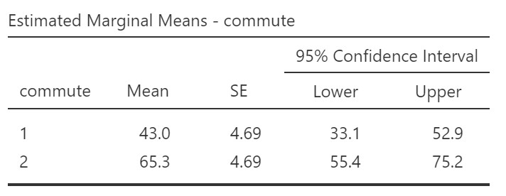
We can compare these values to the descriptive statistics we obtained earlier. For the descriptive statistics the means for driving and cycling were 43.3 and 65.0, respectively. The marginal means are the values computed by the model – the expected values for happiness when controlling for age. That is why the values in the marginal means table are slightly different from the values for the descriptive statistics computed on the raw data.
Finally, let’s write up our results in APA format.
We conducted a study examining how commute affects happiness levels. Furthermore, we collected data on age as a covariate of our study. We satisfied all assumptions of the ANCOVA except that we violated the assumption of homogeneity of regression slopes. Despite failing to meet this assumption, we proceeded with the ANCOVA analysis.
There was a significant effect of commute on happiness, such that people who commuted via cycling (M = 65.3, SE = 4.69, 95% CI [33.1, 52.9]) reported higher happiness than people who commuted via driving (M = 43.0, SE = 4.69, 95% CI [33.1, 52.9]), while controlling for age, F(1, 17) = 11.21, p = .004, ω2 = .33. The relationship between age and happiness was not significant, F(1, 17) = 2.07, p = .17.
