Power

What is power in reference to statistics? It is the probability that your statistical test will detect an effect, given that there is an effect in the population. It can be reported as a number from 0 to 1 or as a percentage, from 0 to 100% As you might have guessed, we want high power! So, how do we achieve high power?

Go to this app and follow the instructions to find out:

https://rpsychologist.com/d3/nhst/

First of all, adjust the settings as follows:

• Solve for? Power
• Significance level α = .05
• Sample size n = 30
• Effect size d = 0.50 (this is sometimes called a medium effect size – more on this later)
• One-tailed test

How much power did you have? (Write it down—the number is a % below the graph)

Now, try the following and observe what happens to the value for power (i.e., does it go up or down?). In each case, write down your answer.

1. Increase the significance level to .10 (i.e., a less stringent α). Then return the significance level to .05.
2. Decrease your sample size to 20.
3. Increase your sample size to 50. Then return the sample size to 30.
4. Decrease the effect size to 0.20 (this is sometimes called a small effect size).

Feel free to play around with these variables some more until you get a sense of how each of them influences power. Now you should be able to fill in the blanks in the following paragraphs:

A very simple way to influence power is to tweak your α. Remember that trade-off between type I and type II error? Well, it turns out that power is related to type II error. In fact, power = 1- β (where β is the probability of making a type II error). So, if you increase your α (i.e., use a less stringent test) then you _______________ power. So using α = .10 instead of .05 will _______________ the power of the test. Of course that comes at a cost of increasing your chance of a type I error, so this is not recommended.

What are some practical ways to influence power?

1. Increasing your sample size will _______________ power.
2. Increasing the size of the effect will _______________ power. Remember how we talked about aiming for a strong manipulation? This will increase the size of the effect and _______________ power.
3. Given what you know about the roles of systematic and unsystematic variation in test statistics, and that “test statistic = signal/noise,” or “test statistic = systematic variation/unsystematic variation” what do you think will happen to power if you reduce that unsystematic variation? Reducing variability will _______________ power.

You might be wondering how much power we should aim for? Well, just as there is no perfect answer to what α level we should use, there is no ideal value for power. However, many researchers agree that 80% is a basic minimum that we should be aiming for. More on this later.

The key takeaway here is that effect size, sample size, alpha, and power are all related. If you know three out of the four of them, you can determine the fourth. Later in this chapter, you’ll learn how to determine the appropriate sample size, given power, alpha, and the effect size of interest to you.

Effect Size

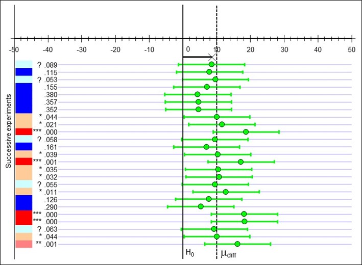
After running an inferential test, it might be tempting to look at the p-value and if p < .05, to call it a day! However, there are some big limitations to looking at p-values alone. Imagine you run a study to test the effects of completing practice test questions on students’ stats exam scores. You are interested in the difference between the mean scores when students either do, or do not, complete the practice test questions. Under the null hypothesis, you expect no difference. Let’s say the true difference in scores is a full 10 percentage points. You run a study with 32 participants but get no significant results. Should you give up your career as a researcher? Not so fast! If you go back and run that same study, with a different sample each time, 25 times, you might get something like this:

Here is a series of replications (i.e., the same study repeated again with different participants from the same population). Each row in the figure represents a replication. In this hypothetical example, the true effect in the population is a medium effect size (d = 0.50). The figure gives us the difference between means under the null hypothesis—the black bar (= no difference between groups)—and the true difference between the mean test scores—the dashed line. The small green circles represent the mean difference for each study, and the green bars extending out from those circles represent the confidence intervals (CIs). If those CIs do not cross the solid black line, then you have a significant result. The p-values are on the very left (remember, they are significant if they drop below .05. Those that are close are marked with a ?).

Note that only 11 of the 25 studies (fewer than half of them) turned out to be significant here! All the means (the circles), are above the value for the null hypothesis, so the effect was in the expected direction for all the studies, but fewer than half were significant. The problem here is that power is only .52, or 52%. And your sample was relatively small at only 32 participants. The overall effect size across these many studies would average out to be about .50 – which is considered a medium effect size. The take-away point here is that just looking at the p-value from one study is not really very meaningful! And this really illustrates why it is important to think about power and effect size. If we repeated the exercise with a larger sample size for each replication (i.e., producing higher power), more of these studies’ results would have been significant. Or, if the effect size in the population had been larger, more of these results would have been significant.

And… if you want to look at another cool visualization that will show you how confidence intervals vary across multiple experiments, go here:

https://rpsychologist.com/d3/ci/

You can adjust the sample size, too, and see how with larger samples, the confidence interval gets smaller and is more likely to include the true population mean (in this example, the true population mean is 0 and is represented by the dashed orange line going up through the middle of the graph).

Hopefully by now you have seen that p­-values alone are not very useful. Remember, too, that they lead you to make these binary decisions—effect significant or not significant—but they do not tell us how big or important the effect is. And, by the way, the p-value is not linearly related to the size of the effect.

Therefore, the American Psychological Association Publication Manual now requires researchers to report effect sizes. An effect size is simply a standardized measure of the size of an effect. You might think that you can just report the difference between your two means (for example) as the effect size. That could be somewhat helpful, but the number obtained would not be easy to compare with results obtained in other studies. Therefore, we compute a standardized measure, which is comparable across studies: it is less reliant on sample size than p-values are, and it takes into account variability in the sample. Below are some of those standardized measures. Effect sizes can be measures of association (like Pearson’s r) or the size of the difference (in standardized units) (like Cohen’s d).

Standardized mean differences

• Cohen’s d is one of the most popular standardized mean difference effect size measures
• Hedges’ g is a less biased version of Cohen’s d. Cohen’s d is problematic for small sample sizes, so Hedge’s g is preferred. Unfortunately, you will not always see it provided in statistical software.

Measures of association:

•  Pearson’s r indicates strength of association and R² indicates proportion of the variance explained.
• η² (eta-squared) measures the proportion of variance in the dependent variable associated with the different groups of the independent variable. This is considered a biased estimate, especially when trying to compare values across studies, so there are two more preferred effect sizes.
• η²_p (partial eta-squared) is calculated slightly differently and is considered a less biased estimate. This can allow for better comparisons of effect sizes across studies. It’s still not perfect, though. You might also come across η²_G (generalized eta-squared) and this is preferred by some authors.
• ω² (omega-squared) is calculated even more differently and is considered the least biased estimate. There is also ω²_p and ω²_G (generalized omega-squared) but we won’t get into that.

(If you nerded out over this information and want to learn more, check out this great and very practical journal article by Daniel Lakens.)

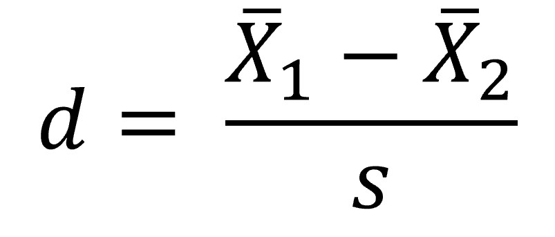
For example, this is how to calculate Cohen’s d. You can use it when you have two means:

How would you interpret the value for r or Cohen’s d? Well, there are some guidelines for r and d:

• r = .1, d = .2 (small effect):
  • the effect explains 1% of the total variance
• r = .3, d = .5 (medium effect):
  • the effect accounts for 9% of the total variance
• r = .5, d = .8 (large effect):
  • the effect accounts for 25% of the variance

We’ll discuss % of total variance more when we get into regression, but essentially it tells us how much variability in the outcome is explained by the predictor. Beware of these ‘canned’ effect sizes though: the size of effect should be placed within the research context. A small effect size might be really important if you are talking about life and death situations. E.g., aspirin reduces the incidence of heart attacks. It’s a small effect – r = .034, R² = .0011 (that is saying that 0.1% of the variance in getting a heart attack is explained by whether or not you take aspirin!). That’s very small, but pretty important in this context, given that aspirin is cheap and with minimal side effects in the adult population.