5 Central Tendency, Dispersion, and Shape
Central Tendency
There are multiple measures of central tendency (these are all averages so you must be careful when you say that word to explain which type you mean!):
- Mode: the most frequent score; the only measure suitable for nominal data; not stable across samples-subject to substantial sampling fluctuation; ignores much information in the data set
- Multimodal or bimodal: when two or more values are the most frequent score
- Median: the middlemost value; less susceptible to outliers and best used when interval/ratio data are skewed; used for ordinal data; moderately stable across samples; loses information (only reflects frequency of scores in the lower half of the distribution)
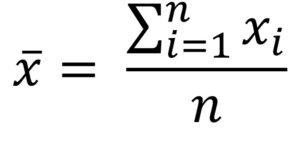
- Mean: the sum of all points divided by the total number of points; susceptible to outliers; stable across samples; see below, where xi represents an individual score in the dataset, Σ represents sum, and n is the number of scores in the dataset.
The mean

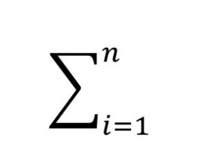
This formula can be a bit overwhelming, at first glance! What you need to know is that this symbol Σ (sigma) means “sum of.” And

means: add these things together, from i = 1 (the first participant) to n = the last participant in the dataset.
Dispersion
The mean on its own does not tell us very much. Perhaps everyone scored the mean, or perhaps there was lots of variability in scores around the mean. Therefore, we also look at something called dispersion, which relates to how much our scores are spread out in our dataset. There are multiple measures of dispersion.
- Range: the difference between the maximum and minimum value (e.g., if the minimum score is 17 and the maximum is 49, then the range is 32)
- Quartile: when a dataset is divided into four equal parts, the first quartile (Q1) is at the 25th percentile, the second quartile (Q2) is at the 50th percentile, and the third quartile (Q3) is at the 75th percentile.
- Interquartile range: the middle 50% (Q1 to Q3)
- Variance: the sum of the squared deviations from the mean. This means first (a) calculating the mean, (b) subtracting each score from the mean (aka deviations from the mean), (c) squaring each of those deviations values, and (d) summing all those squared deviations. This is represented by the equation:
![]()
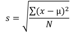
- Standard deviation: is the square root of the variance. This is represented by the equation:

-
- equations are only used if we are examining the whole population. If we only have a sample, we replace the denominator N with N-1.
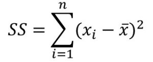
- You should also be aware of the sum of squared errors (SS). This reflects the total spread of scores around the mean:

- Note that we do not use SS as a measure of descriptive statistics because the size of SS depends on the number of scores in the dataset. If we take an average of SS, we get variance. Variance is not that useful as a descriptive statistic because it is measured in units squared. Therefore, we usually report the standard deviation (square root of the variance). The standard deviation can be used to compare variation across different sized samples because it represents a “standardized” amount of deviation from the mean.
- However, we do use SS in inferential statistics, so you will see it again later!
- Finally, SS, variance, and standard deviation all tell us:
- How well the mean “fits” the data – smaller values indicate better fit
- Variability of the data
- How well the mean represents the observed data
- How much “error” there is
Shape
Finally, there are two main measures of shape that describe the shape of the distribution of our data:
- Skew: in a non-normal distribution, it is when one tail of the distribution is longer than another, producing an asymmetric distribution.
- Negative skew: when the tail points to the negative end of the spectrum; in other words, most of the values are on the right side of the distribution
- Positive skew: when the tail points to the positive end of the spectrum; in other words, most of the values are on the left side of the distribution
- Kurtosis: the weight of the tails relative to a normal distribution.
- Leptokurtic: light tails; values are more concentrated around the mean
- Platykurtic: heavy tails; values are less concentrated around the mean
There are other terms we use to describe data:
- Frequency distribution: overview of the times each value occurs in a dataset; often portrayed visually like with a histogram
- Histogram: a visual depiction of the frequency distribution using bars to depict a range of the distribution
- Normal distribution: a special distribution in which the data are symmetrical on both sides of the mean; under a normal distribution, the mean is also equal to the median
