40 Fit of the Regression Model
Model Fit
When we have created our regression line, we want to know how well this model fits the data. In some cases, when the datapoints are all very close to the regression line, the model fits the data very well. In other cases, when the datapoints are scattered more widely around the regression line, the model does not fit the data as well. We can quantify this fit in two ways: R2 and F. Before computing these, we need to look at sums of squares in regression:
You may recall that in the chapter on one-way ANOVA, we said that:
The total variance, sum of squares total, SSt, is an indication of how much all the scores in the experiment vary around the grand mean (i.e., the mean of all the scores). The model sum of squares, SSm, sometimes reported as SSb (between-groups sum of squares, for the one-way ANOVA) reflects how much the group means vary around the grand mean. And the residual sum of squares, SSr, reflects how much participant scores vary around their own group means. So, SSr is the amount of variability that is left over when we use the model (i.e., the group means) to predict scores, compared to when we just use the grand mean to predict scores.
You might be wondering how this works with regression in the case where we have a continuous predictor. It can help to visualize it. Let’s take our mother grumpiness data again. To simplify things for the example, we’ll just look at a subset of the data (5 data points), but in reality, all this would actually apply to the whole dataset. In each image below, the blue dots represent each participant’s datapoint (X = sleep, Y = grumpiness). The horizontal red line represents the mean grumpiness.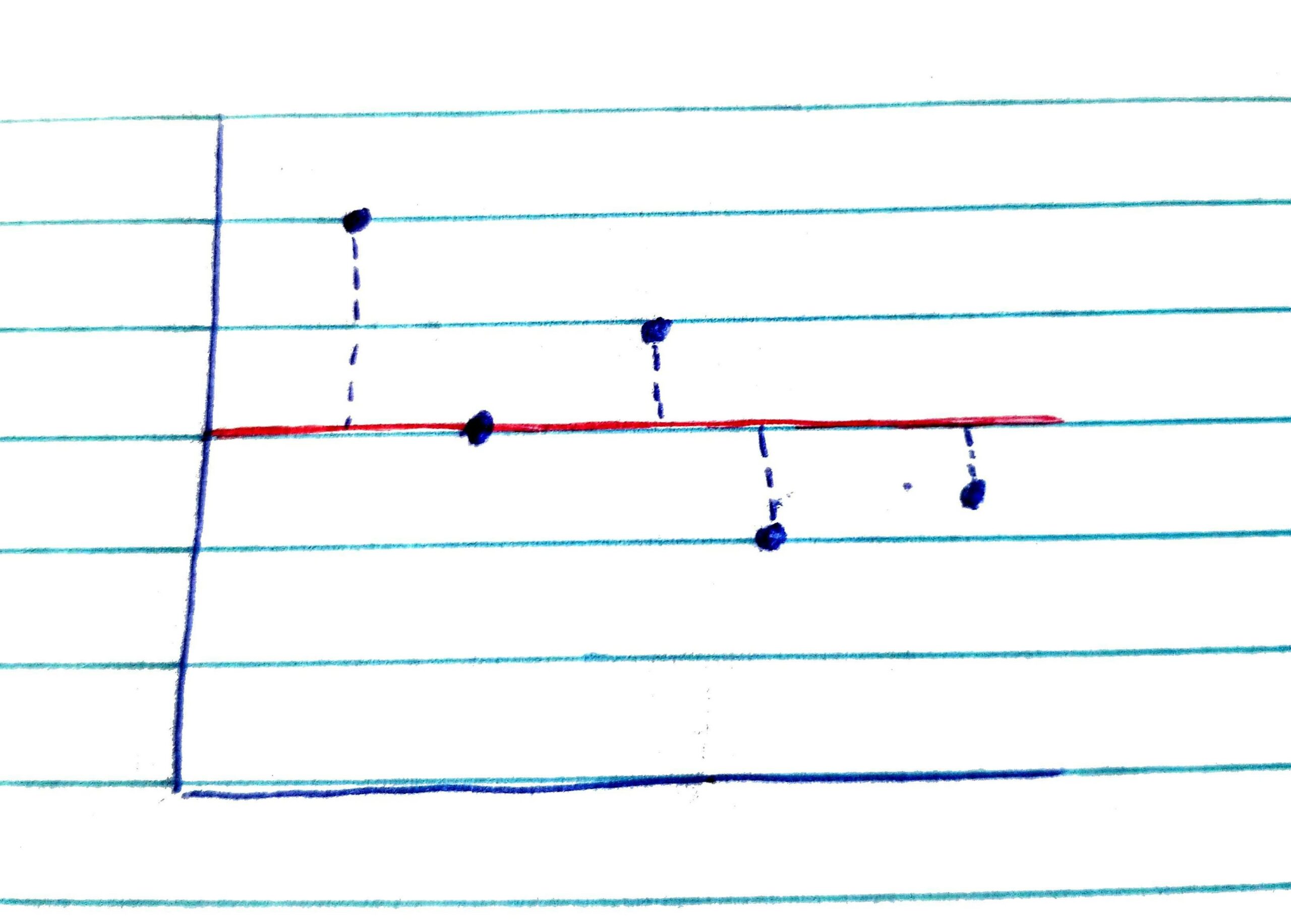
SSt First, let’s imagine a situation where we just use the mean grumpiness scores as our predictor of Y. In other words, if we wanted to predict a grumpiness score in the dataset, we imagine that we do not know anything about the predictor (sleep). If we do not know anything about the predictor, the best information we have to go on if we want to guess what the grumpiness score might be on any given day is the mean of the grumpiness scores. The dashed lines between the datapoints and the red line for the mean grumpiness scores indicate how much error there would be if we used the mean of Y to predict Y scores. If we square and sum those squared errors, we compute SSt, or the total sum of squares. SSt tells us how much error there is if we just use the mean of Y to predict Y-scores. SSt indicates the amount of variability of the Y scores around the mean of Y.
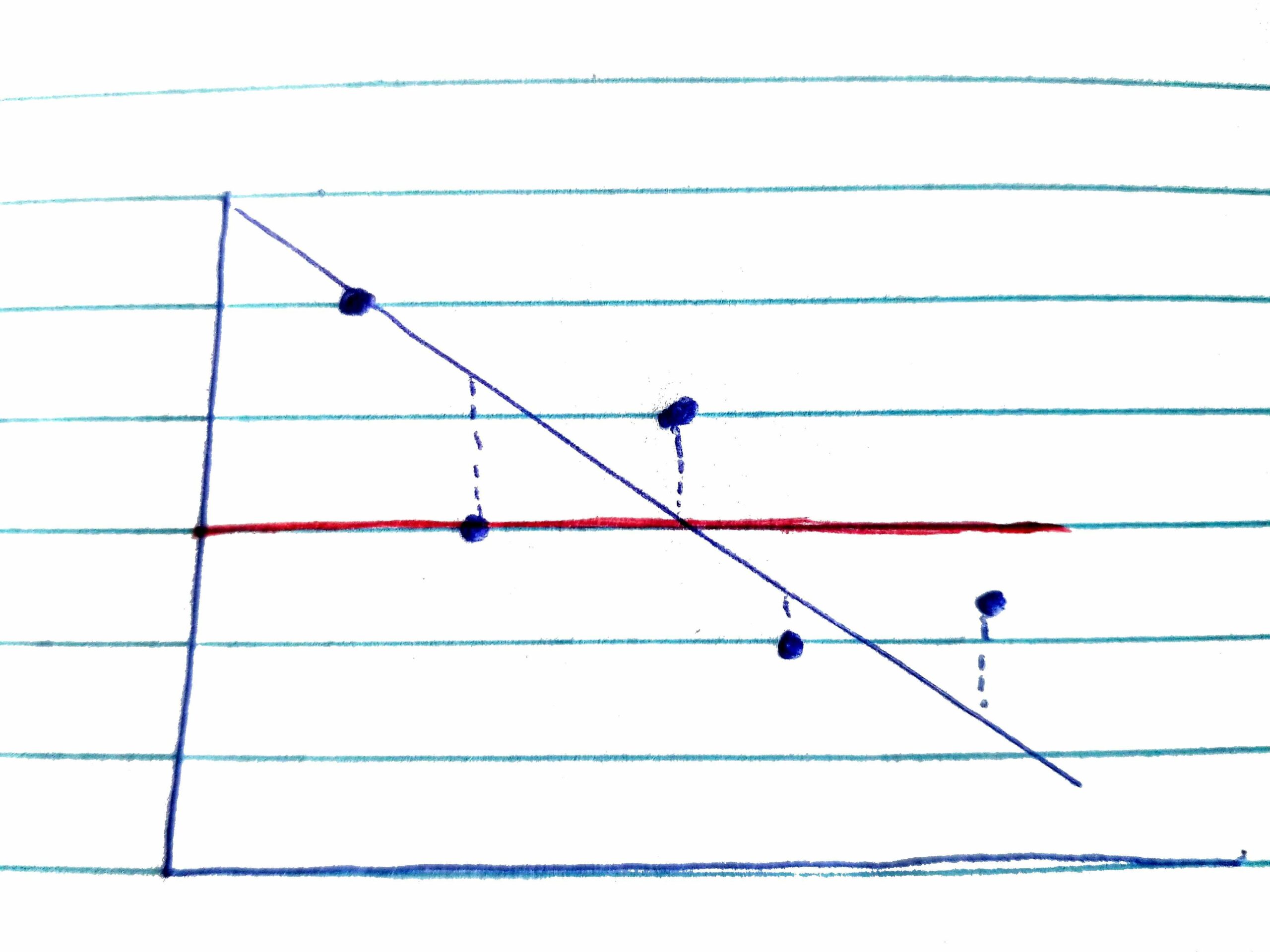
SSr Next, let’s imagine we use the regression line to predict scores. We (or, in our case, jamovi) finds the best fit line. However, unless there is a perfect relationship between X and Y (a highly unlikely scenario) the datapoints will not lie on the regression line, but above and below it. The vertical distance between each datapoint and the regression line (indicated by the dashed lines in this figure) is the residual. SSr, the sum of the squared residuals, indicates the amount of error we have when we used the regression line to predict the Y-scores. SSr indicates the amount of variability of the Y scores around the regression line.
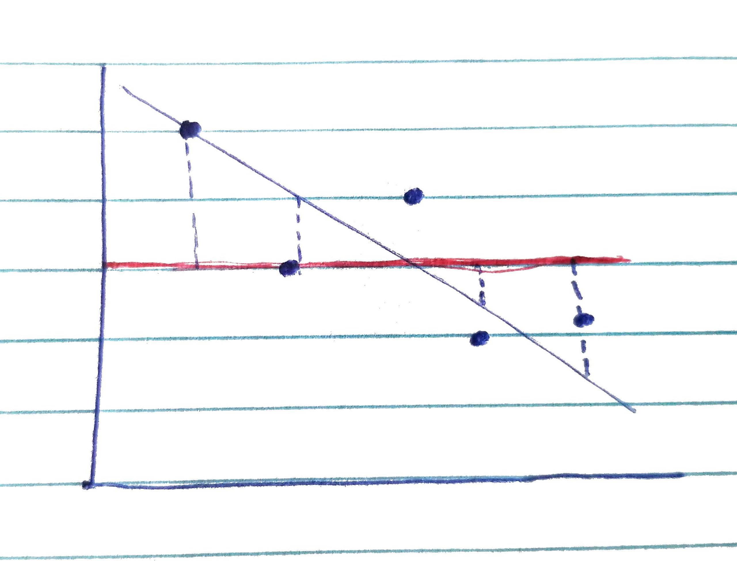
SSm Finally, we can measure the distance between the regression line (the predicted Y-values) and the mean of Y, for each datapoint. SSm is the sum of those squared values – the model sum of squares. SSm reflects the amount by which error is reduced by using the model (the regression line) to predict Y-scores instead of using the mean of Y to predict Y-scores. Again, remember that we are using regression to be able to predict Y, from X. SSm tells us how much improvement we get in our predictions when we use the predictor to predict Y-scores, compared to when we just use the mean of Y to predict Y-scores.
We can use SSt, SSr, and SSm in different ways to assess the fit of the model, the regression line, to the data.
Model Fit: R2
One measure of model fit is R2. R2 represents the proportion of the variance in Y, the outcome, accounted for by the regression model. In the case where there is just one predictor, it is the proportion of the variance in Y explained by the X, the predictor. It is computed as follows:
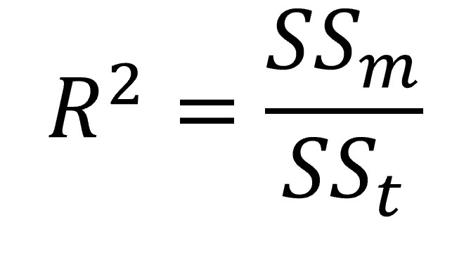 As you can see from the equation, R2 is calculated as the variance explained by the model, divided by the total variance (around the mean of Y) – hence, proportion of the variance!
We can write this value as calculated, or convert it to a percentage by multiplying by 100. For example, it is acceptable to write either R2 = .36 or R2 = 36%. This is considered to be a measure of effect size.
Model Fit: F
Another way to quantify model fit is to compute F. As we saw in the earlier chapters on ANOVA, F is computed as follows:
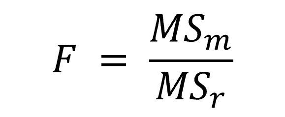 In other words, F the improvement due to the model, divided by the amount of error that is remaining (the difference between the model and the observed data). If we have a good model, with all the datapoints close to the dotted line, then MSm will be large and MSr will be small, and so F will be large. We can test if the F is significant (jamovi will do this for us). If it is significant, we shall conclude that the model fits the data well and that the regression line does a good job of describing the relation between X and Y.
Testing Individual Predictors
We can also test whether individual predictors in our model are significant predictors of the outcome. This is particularly useful when we have multiple regression (i.e., when there is more than one predictor variable), because we can test the extent to which an individual predictor predicts the outcome, while controlling for all other predictors in the model. However, we can also do this for simple regression (i.e., with one predictor), but the results in this case will just tell us the same as the F.
You will recall that our regression model looks like this:
Yi = (b0 + b1Xi ) + errori
You may also remember that b1 is the slope of the regression line (for each unit increase in X, by how many units does Y increase). We can test if the b1 in our model is significantly different from zero. If our best fit line is just a horizontal line through the dataset (like the red line for the mean, earlier in this section), then, the value of b1 is going to be zero. The more Y changes with each change in X, the more the value for will b1 move away from zero (either becoming more positive or more negative), and at some point it will be significantly different from zero. You will see that in jamovi we can run a t-test to test if the b1 slope is significantly different from zero.
