23 In Practice: One-Way ANOVA
Let’s take a look at how to run the one-way ANOVA using jamovi.
Remember our four steps to data analysis:
- Look at the data
- Check assumptions
- Perform the test
- Interpret results
1. Look at the Data
For this chapter, we’re going to work with example data from lsj-data. Open data from your Data Library in “lsj-data.” Select and open “clinicaltrial” (not Clinical Trial 2). This dataset is hypothetical data of a clinical trial in which you are testing a new antidepressant drug called Joyzepam. In order to construct a fair test of the drug’s effectiveness, the study involves three separate drugs to be administered. One is a placebo, and the other is an existing antidepressant / anti-anxiety drug called Anxifree. A collection of 18 participants with moderate to severe depression are recruited for your initial testing. Because the drugs are sometimes administered in conjunction with psychological therapy, your study includes 9 people undergoing cognitive behavioral therapy (CBT) and 9 who are not. Participants are randomly assigned (doubly blinded, of course) a treatment, such that there are 3 CBT people and 3 no-therapy people assigned to each of the 3 drugs. A psychologist assesses the mood of each person after a 3 month run with each drug, and the overall improvement in each person’s mood is assessed on a scale ranging from -5 to +5.
Data Set-Up
To conduct the one-way ANOVA, we first need to ensure our data is set-up properly in our dataset. This requires having two columns: one with our continuous dependent variable and one indicating which group the participant is in. Each row is a unique participant or unit of analysis.
Note that in this dataset we actually have two independent variables: drug and therapy. If we were looking at the effect of therapy on mood.gain (our DV) then we would only need to perform an independent samples t-test because there are only two groups (no.therapy and CBT). However, if we were looking at the effect of drug on mood.gain, which is our goal in this chapter, then we would perform a one-way ANOVA because there are three groups (placebo, anxifree, and joyzepam).
Describe the Data
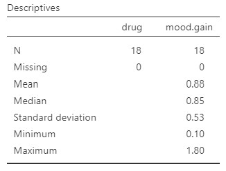
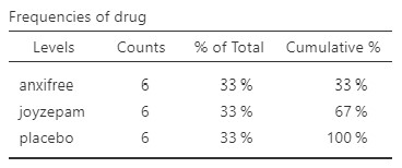
Once we confirm our data is setup correctly in jamovi, we should look at our data using descriptive statistics and graphs. First, our descriptive statistics are shown below. We see that there are 18 cases in our dataset (a bit small, but let’s ignore that for now) with no missing data. The mean mood gain was .88 (SD = .53) with a minimum mood gain of .10 and maximum of 1.80. Furthermore, there are 6 people in each of our three conditions in the study so we have a balanced research design.
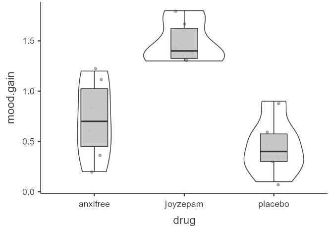
In addition, we may want to look at the distribution of mood gain across our three conditions. In the Descriptives analysis, we can choose to “split by” drug and then ask for a box plot with violin and data points like below. Visually, it seems like joyzepam might be leading to greater mood gain than the other two conditions, but we need to analyze it statistically to know for sure!
Specify the Hypotheses
Our basic research question for the one-way ANOVA is whether there is a difference in mood between the three drugs. Therefore, our null hypothesis would be that there is no difference in mood between the three drugs, and the alternate hypothesis would be that there is a difference in mood between the three drugs.
2. Check Assumptions
As a parametric test, the one-way ANOVA has the same assumptions as other parametric tests:
- The dependent variable is normally distributed
- Variances in the two groups are roughly equal (i.e., homogeneity of variances)
- The dependent variable is interval or ratio (i.e., continuous)
- Scores are independent between groups
We cannot test the third and fourth assumptions; rather, those are based on knowing your data.
However, we can and should test for the first two assumptions. Fortunately, the one-way ANOVA in jamovi has three check boxes under “Assumption Checks” that lets us test for both assumptions. Note that all the same caveats to interpreting the assumption checks (which we noted with in the chapter on t-tests ) also apply in the case of one-way ANOVA (review that section if need be!).
ANOVA is (Somewhat) Robust to Violations
Although we should attend to the assumptions, in general the F-statistic is robust to violations of normality and homogeneity of variance. This means that you can still run the one-way ANOVA if you violate the assumptions, but only when group sizes and variances are equal or nearly equal. If you have vastly different variances (such as 2:1 ratio or greater) or vastly different group sizes (such as a 2:1 ratio or greater), and especially if one group is really small (e.g., 10 or fewer cases), then your F-statistic is likely to be very wrong. For example, if your larger group has the larger variance, then your F-statistic is likely to be non-significant or smaller than it should be; however, if your larger group has smaller variance, then your F-statistic is likely to be significant or bigger than it should be! Thus, you might either conclude there is no effect when there is indeed one in the population, or vice versa. In these situations, you can use the Walrus package in jamovi (it’s an add-on so you will need to add it manually and select the Robust ANOVA), or you can use a non-parametric test (described later in this chapter).
If you select ANOVA in jamovi and then choose the ANOVA (not the One-Way ANOVA option – we shall not use that for this class), you can select the assumption checks Homogeneity test, Normality test, and Q-Q plot.
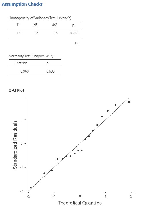
The Shapiro-Wilk test was not statistically significant (W = .96, p = .605); it might appear that we can conclude that the data are normally distributed. However, as previously discussed, this test is going to be non-significant even with significant deviations from normality when we have a small sample size, and, when we have such a small sample size, we cannot assume that central limit theorem applies. Similarly, for Levene’s test of homogeneity of the variances: it is not significant, but this might be because we have such a small sample size.
The table below shows some options for alternative tests when assumptions are not satisfied (or when we cannot conclude they are satisfied because we have a very small sample size).
| Normality: satisfied | Normality: not satisfied | |
| Homogeneity of the variance: satisfied | One-way ANOVA (using the ANOVA function) | Kruskal-Wallis test or robust ANOVA (Walrus package) |
| Homogeneity of the variance: not satisfied | Welch’s F-test (using the one-way ANOVA function) | Kruskal-Wallis test or robust ANOVA (Walrus package) |
With our clinical trial data, given that we have such a small sample size, I would go to a non-parametric test, but for illustrative purposes, let’s first perform the ANOVA.
3. Perform the Test
I recommend using the ANOVA analysis in jamovi. Do not use the One-Way ANOVA analysis, unless you need Kruskal-Wallis or Welch’s F-test – the options are too limited for our purposes.
In our example, the researcher did not have specific hypotheses about which groups would differ from each other so we should use post hoc tests to obtain all the possible pair-wise comparisons. For illustrative purposes, I am also going to run planned comparisons as well. In this case, I am going to run a simple contrast to compare joyzepam with placebo and anxifree with placebo. Note that we would only run these contrasts if we have specific predictions about which groups will differ from each other, and that we need to apply an appropriate correction if we use non-orthogonal comparisons (see previous section of this chapter!).
- To perform a one-way ANOVA in jamovi, go to the Analyses tab, click the ANOVA button, and choose “ANOVA.”
- Move your dependent variable to the Dependent Variable box and your independent variable to the Fixed Factors box. In this case, move
mood.gainto the Dependent Variable box anddrugto the Fixed Factors box. - Select ω2 (omega-squared) for your effect size.
- Ignore the Model drop-down menu. If you are doing more complicated ANOVAs you will need this. We will ignore it.
- In the Assumption Checks drop-down menu, select all three options:
Homogeneity test,Normality test, andQ-Q plot. - To obtain post hoc tests, under the Post Hoc Tests option, move the independent variable over to the box on the right, and select both Holm, Bonferroni, and No correction (note, we would not normally select multiple post hoc tests, but this will allow you to see how they vary in their consequences for the p-value). In addition, check the box for Cohen’s d, to obtain a measure of effect size. To obtain contrasts, under “contrasts,” click on the drop-down menu to the right of the independent variable in question and select the contrast you would like. For this example, choose a simple contrast.
- In the Estimated Marginal Means drop-down menu, move your IV
drugto the Marginal Means box and selectMarginal means plots,Marginal means tables, andObserved scores, in addition to the pre-selectedEqual cell weights.
4. Interpret Results
Once we are satisfied we have satisfied the assumptions for the one-way ANOVA, we can interpret our results.
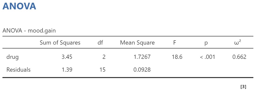
The result shows a significant ANOVA and we would follow-up by looking at the post hoc tests or planned comparisons as appropriate. Below is the table showing the results of the Post Hoc Tests in jamovi.

Remember that, normally, we should select the appropriate post hoc test based on our data, rather than running three different tests. However, by running these three tests, you can see how they differ in the output they provide. You will notice that the p-value changes according to whether you look at the first p (which is for the comparison with no correction), the Bonferroni, or the Holm test. Bonferroni results in the largest p-value and is the most conservative. In our example, Holm and no correction result in the same p-value. In some scenarios, Holm will result in smaller p-values than no correction (because it involves some correction and so is less powerful than applying low correction). If we had elected to use Holm, we would note that there is a significant difference between placebo and joyzepam, and also between anxifree and joyzepam, but not between placebo and anxifree. We can look at the graph to verify the direction of the effect.
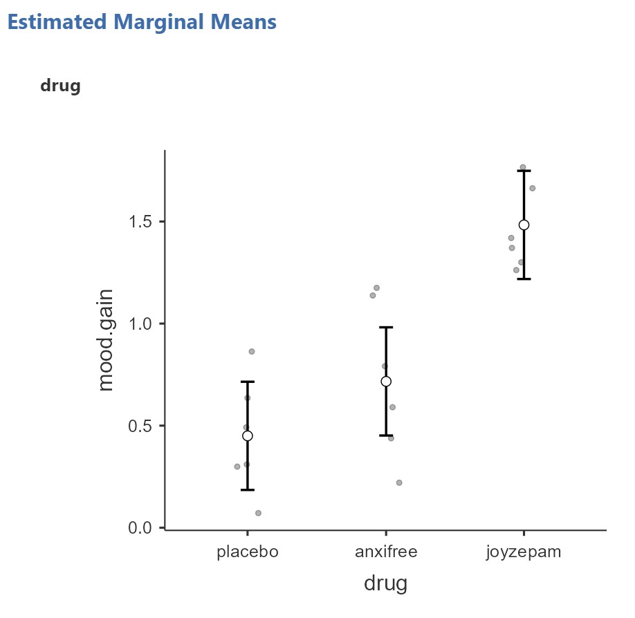
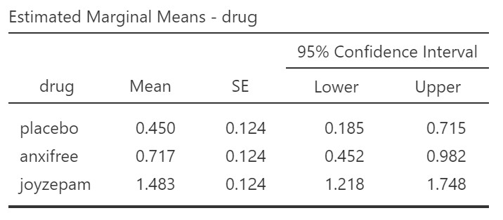
You can see from the marginal means that it is that joyzepam show higher mood gain scores than anxifree and placebo.
Let’s say, instead, that you had some specific predictions that both joyzepam and anxifree would result in higher mood gain scores than placebo. In this case, you have planned comparisons, and so you would look at the contrasts results in jamovi. The results for the simple contrasts are below.
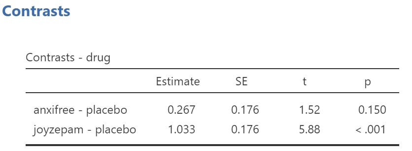
As described in the previous section of this chapter, simple contrasts are non-orthogonal comparisons. Therefore, we would need to apply a correction to the p-value ourselves. You can use the Bonferroni correction, dividing α by two, because we conducted two tests for the contrasts. Therefore, α = .05/2 = .025. By this criterion, joyzepam results in significantly higher mood gain scores than placebo, but anxifree does not.
Write up the results
In APA format, and reporting on the results of the post hoc tests, we could say something like this:
There was a significant difference in mood gain across the three drug conditions, F(2, 15) = 18.61, p < .001, ω2 = .66. Participants who received joyzepam had higher mood gain scores (M = 1.48, SE = 0.12, 95% CI [1.22, 1.75]) than participants who received either anxifree (M = 0.72, SE = 0.12, 95% CI [0.45, 0.98]), or placebo (M = 0.45, SE = 0.12, 95% CI [0.19, 0.72]), t(15) = 4.36, pholm = .001, d = 2.52, and t(15) = 5.88, pholm < .001, d = 3.39, respectively. However, there was no significant difference between participants who received anxifree compared to those who received placebo, t = 1.52, pholm = .15.
If we instead wanted to report the contrasts (note, we would only do this if we had specified these as planned comparisons a priori), we could report as follows (the contrasts do not give me a Cohen’s d so I can obtain that by looking at the post hoc test results):
There was a significant difference in mood gain across the three drug conditions, F (2, 15) = 18.61, p < .001, ω2 = .66. I used planned comparisons to compare mean mood gain scores for participants in the anxifree and joyzepam groups to the placebo group, applying the Bonferroni correction (α = .05/2 = .025). Participants who received joyzepam had higher mood gain scores (M = 1.48, SE = 0.12, 95% CI [1.22, 1.75]) than participants who received placebo (M = 0.45, SE = 0.12, 95% CI [0.19, 0.72]), t = 5.88, p < .001, d = 3.39, but participants who received anxifree (M = 0.72, SE = 0.12, 95% CI [0.45, 0.98]) did not have higher mood gain scores than participants who received placebo, t = 1.52, p = .15.
Note that in this situation, whether we use the post hoc tests or the contrasts, the results turn out the same. However, this will not always be the case. Therefore, you should always decide prior to conducting your analyses whether you are going to look at the post hoc tests or whether you have specific contrasts of interest (based on prior research and/or theory) and will use planned comparisons, i.e., contrasts.
Finally, what would we write up if the ANOVA result itself was not significant? In that case, we would not report follow-up tests (whether we had planned comparisons or were going to use post hoc tests).
